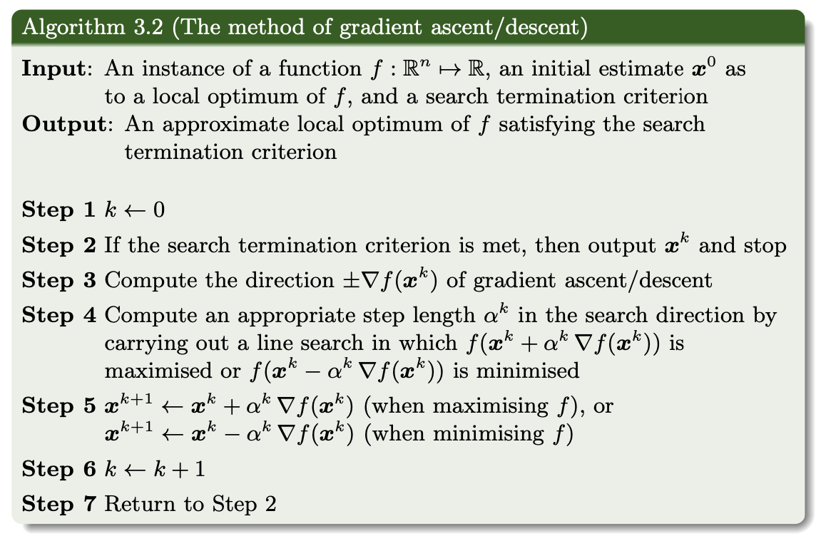
Method of Gradient Descent

Method of Gradient Descent

Similar to Method of Gradient Ascent Also see Gradient Ascent

Consider the function

$$f(x_1,x_2)=x_1^2+3x_2^2+2x_1{x}_2-4x_1-6x_2$$

with initial estimate

$$\text{x}={\left[\begin{array}{cc}0& 0\end{array}\right]}^T$$

Calculate the gradient vector

$$▽f(\text{x})={\left[\begin{array}{cc}2x_1+2x_2-4& 6x_2+2x_1-6\end{array}\right]}^T$$

and the Hessian Matrix

$${▽}^{2}f(\text{x})=\left[\begin{array}{cc}2& 2\\ 2& 6\end{array}\right]$$

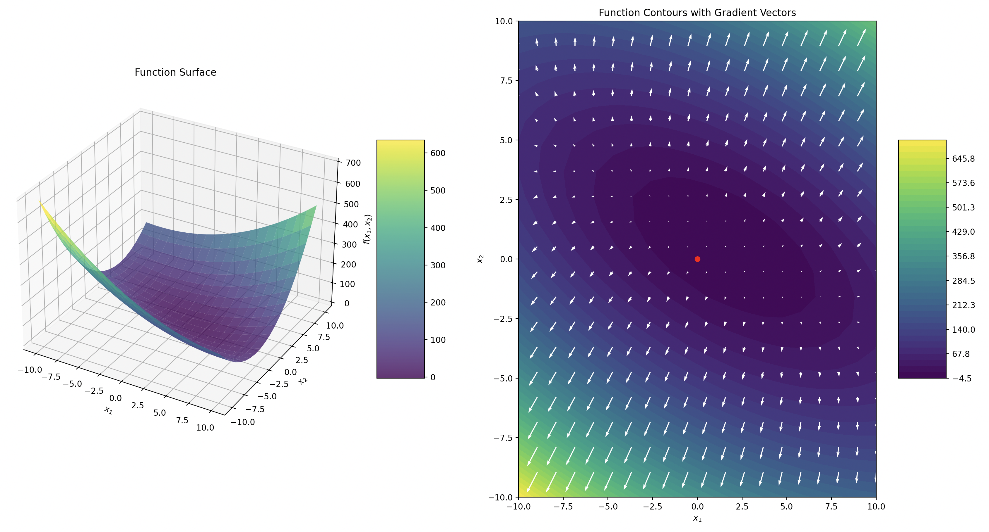
Look at the plot

Do one step of gradient descent:

$f({\text{x}}^0-{\alpha }^0▽f({\text{x}}^0))=\left[\begin{array}{cc}4{\alpha }^0& 6{\alpha }^0\end{array}\right]$

The general gradient descent algorithm for any function with a minimum.

def gradient_descent(func, x0):
 
"""
 
Performs one step of gradient descent with optimal alpha calculation
 
for a given sympy function of x1 and x2, starting from x0.
 
  
 
Parameters:
 
- func: sympy function of two variables, x1 and x2.
 
- x0: Initial point as a list or tuple of two numbers [x1, x2].
 
  
 
Returns:
 
- New point as a list [x1, x2] after one step of gradient descent.
 
- Optimal alpha used for the step.
 
"""
 
# Define symbols
 
x1, x2, alpha = symbols('x1 x2 alpha')
 
# Calculate gradient
 
grad = [diff(func, var) for var in [x1, x2]]
 
# Substitute x0 into gradient and express new point as function of alpha
 
grad_at_x0 = [g.subs([(x1, x0[0]), (x2, x0[1])]) for g in grad]
 
x1_new = x0[0] - alpha * grad_at_x0[0]
 
x2_new = x0[1] - alpha * grad_at_x0[1]
 
# Function value as a function of alpha
 
f_alpha = func.subs([(x1, x1_new), (x2, x2_new)])
 
# Derivative of function with respect to alpha and solve for optimal alpha
 
df_dalpha = diff(f_alpha, alpha)
 
optimal_alpha_solution = solve(df_dalpha, alpha)
 
# Handle multiple solutions for alpha
 
if not optimal_alpha_solution:
 
print("No solution found for alpha. Check the function's form.")
 
return x0, None # Return original point and None for alpha if no solution
 
optimal_alpha = optimal_alpha_solution[0] # Assuming the first solution is optimal
 
# Calculate new point using the optimal alpha
 
x1_optimal = x1_new.subs(alpha, optimal_alpha)
 
x2_optimal = x2_new.subs(alpha, optimal_alpha)
 
return [x1_optimal, x2_optimal], optimal_alpha

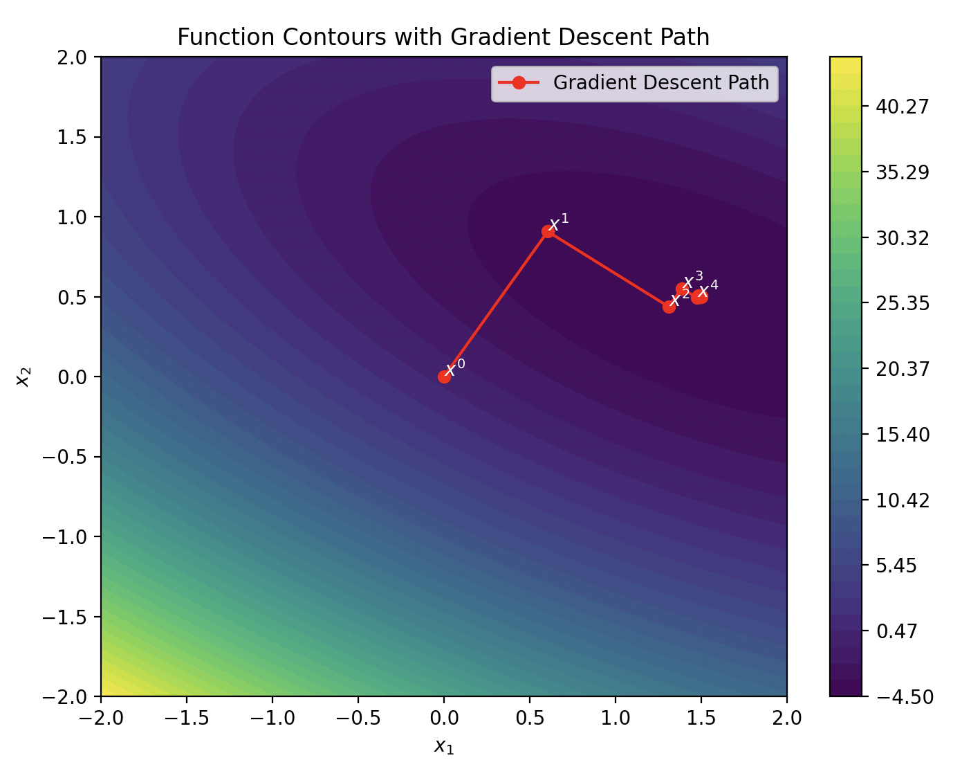
For the function considered, this code will return ${\alpha }^0=\frac{13}{86}$ which will result in the next estimate ${\text{x}}^1={\left[\begin{array}{cc}\frac{26}{43}& \frac{39}{43}\end{array}\right]}^T\approx {\left[\begin{array}{cc}0.604651& 0.906977\end{array}\right]}^T$ Continue doing gradient descent steps until it converges to the approximate global minimum $\text{x}\approx {\left[\begin{array}{cc}1.5& 0.5\end{array}\right]}^T$