Newton Univariate Method

Newton Univariate Method

We firstly considered Newton Univariate Root Method, now we’re looking at Newton’s univariate optimisation method.

Aim:

• Find the local optimum i.e. the x-value that maximises/minimises the function

General Form:

• General formula for Newton’s Univariate Root approximation:

$$x^{k+1}=x^k-\frac{f^{\prime }(x^k)}{f^{\prime \prime }(x^k)}$$

from sympy import symbols, diff, lambdify, parse_expr
 
x = symbols('x')
 
def newton_uni_method(f_sym, x0, tolerance=0.0005, max_iterations=100):
 
	# Convert symbolic function to a numerical function
	f = lambdify(x, f_sym, 'numpy')
	df_sym = diff(f_sym, x)
	df = lambdify(x, df_sym, 'numpy')
	ddf_sym = diff(df_sym, x)
	ddf = lambdify(x, ddf_sym, 'numpy')
 
	results = []
	k = 0
	xk = x0
 
	while k < max_iterations:
		f_xk = f(xk)
		df_xk = df(xk)
		ddf_xk = ddf(xk)
 
	# Avoid division by zero
	if ddf_xk == 0:
		raise ValueError(f"Zero second derivative. No solution found at x = {xn}")
 
	# Newton univariate method update
	delta = - df_xk / ddf_xk
	xk1 = xk + delta
 
	results.append((k, xk, df_xk, ddf_xk, delta, xk1))
 
	if abs(xk1 - xk) < tolerance:
		break
	  
		xk = xk1
		k += 1
 
	return results

Example

Use the same example as used in Newton Univariate Root Method for comparison.

$$f(x)=1+2x^2-e^x$$

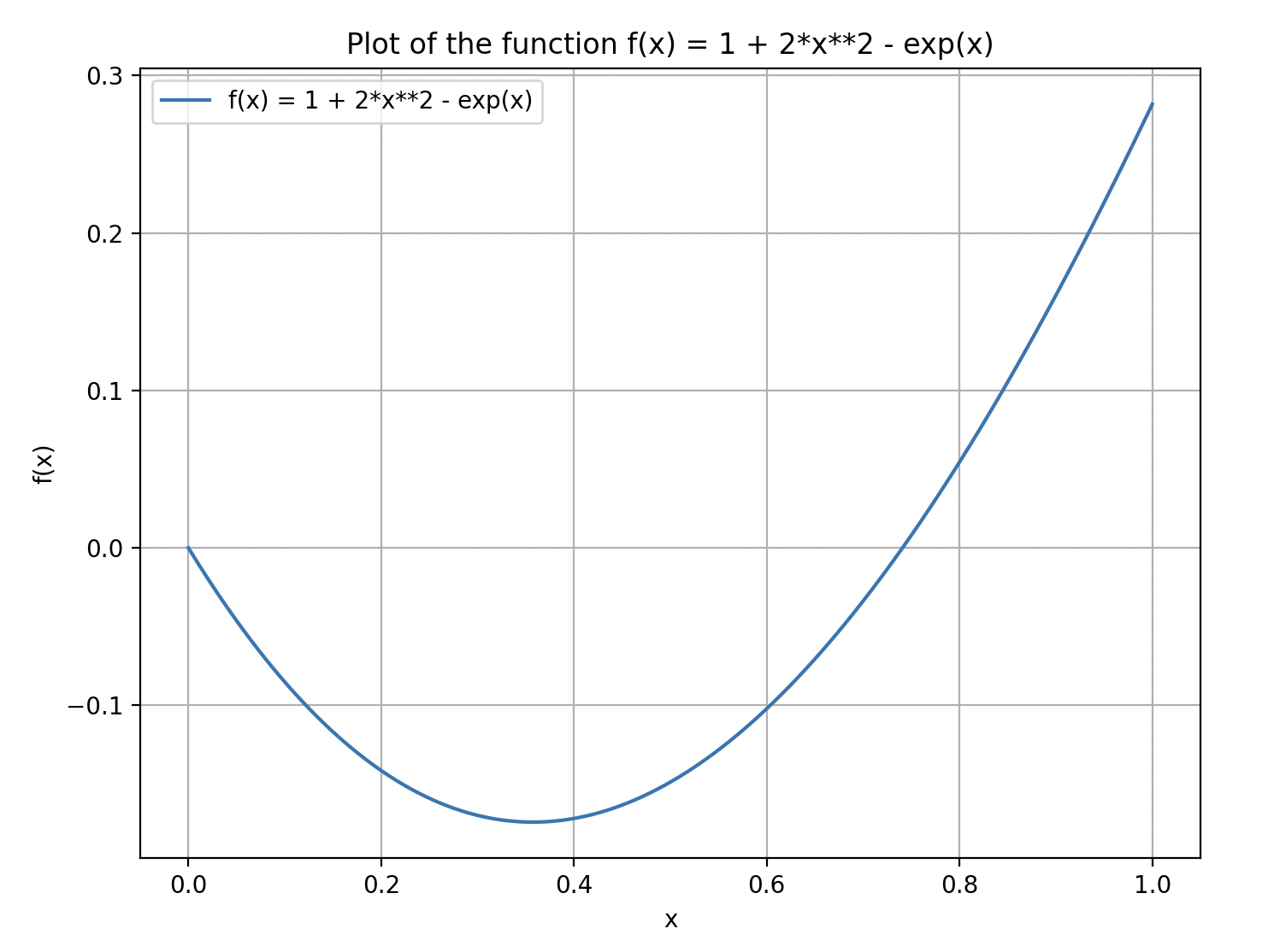From looking at the graph, good initial guesses will be 0.2, 0.4 or 0.6 but the graph might be too much of a hassle to draw. In this case it was given that an initial guess of x = 0.5 must be used.

$k$	$x^k$	$f^{\prime }(x^k)$	$f^{\prime \prime }(x^k)$	$\Delta (x^k)$
0	0.5	0.351 279	2.351 279	-0.149 399
1	0.350 601	-0.017 517	2.580 079	0.006 789
2	0.357 390	-0.000 033	2.570 406	0.000 013
3	0.357 403	-	-	-

using a tolerance of 0.0005 to stop the algorithm results in $x^{\ast }\approx 0.357403$ Comparing the $x^{\ast }\approx 0.357403$ to the graph, we can see that the value obtained is plausible to be the x-value that will result in a local minimum.

Next we’re going to look at Newton Multivariate Method