Intro to Time Series Analysis

Table of Contents

Intro to Time Series Analysis

Chapter 1: The Forecasting Perspective

1.1 Why forecasting?

1.2 An overview of forecasting techniques

1.2.1 Explanatory versus time series forecasting

1.3 The basic steps in a forecasting task

Chapter 2: Basic Forecasting Tools

2.1 Time series and cross-sectional data

2.2 Graphical summaries

2.2.1 Time plots and time series patterns

2.2.2 Seasonal plots

2.2.3 Scatterplots

2.3 Numerical summaries

2.3.1 Univariate Statistics

2.3.2 Bivariate Statistics

2.3.3 Autocorrelation

2.4 Measuring forecast accuracy

2.4.1 Standard statistical measures

2.4.2 Out-of-sample accuracy measurement

2.4.3 Comparing forecast methods

2.4.4 Theil's U-statistic

2.4.5 ACF of forecast error

2.5 Prediction intervals

2.6 Least squares estimates

2.7 Transformations and adjustments

2.7.1 Mathematical transformations

2.7.2 Calendar adjustments

2.7.3 Adjustments for inflation and population changes

Chapter 3: Time Series Decomposition

3.1 Principles of decomposition

3.1.1 Decomposition models

3.1.2 Decomposition graphics

3.2 Moving Averages (MA)

3.2.1 Simple moving averages

3.2.2 Centered moving averages

3.2.3 Double moving averages

3.2.4 Weighted moving averages

3.3 Local Regression Smoothing

3.3.1 Loess

3.4 Classical decomposition

3.4.1 Additive decomposition

3.4.2 Multiplicative decomposition

3.5 STL decomposition

Chapter 4: Exponential Smoothing Methods

Chapter 7: The Box-Jenkins Methodology for ARIMA Models

Chapter 1: The Forecasting Perspective

Why forecasting?

An overview of forecasting techniques

Explanatory versus time series forecasting

The basic steps in a forecasting task

Step 1: Problem definition

What do we want to forecast?
This is sometimes difficult and requires the forecaster to do a lot of research about:
- Who wants the forecasts
- What needs to be forecasted
- How to get the data
It is important to have a clear goal about what you want to achieve

Step 2: Gathering information

It is necessary to obtain past data once you have defined your problem.
This data is used to fit the forecasting model.
Other information about the process may play an important role as well. e.g special events like an economic crisis, public holidays, technological advances etc.
These events often occur as spikes in the time series, and we need to take them into account when fitting a forecasting model.

Step 3: Prelimary (exploratory) analysis

What do the data tell us?
Are there interesting patterns (trends, cycles, seasonality, outliers etc.)
Once we have the data, we would like to make some graphical and numerical summaries to understand the data a bit better.
Such methods will be discussed in Chapter 2 Basic Forecasting Tools and Chapter 3 Time Series Decomposition.
Identifying any patterns are useful in choosing the correct forecasting method.

Step 4: Choosing and fitting models

This step involves choosing and fitting several quantitative forecasting models. We will discuss only exponential smoothing methods (Chapter 4 Exponential Smoothing Methods) and Box-Jenkins ARIMA models (Chapter 7 The Box-Jenkins Methodology for ARIMA Models).

Step 5: Using and evaluating a forecasting model

Once a model has been chosen and its parameters estimated, the model is to be used to make forecasts, and the users of the forecasts will be evaluating the pros and cons of the model as time progress.
A forecasting assignment is not complete when the model has been fitted to the known data.
The performance of the model can only be properly evaluated after the data for the forecast period have become available.

#| label: Assignment 1
Elec <- c(
  1254, 1290, 1379, 1346, 1535, 1555, 1655, 1651, 1500, 1538,
  1486, 1394, 1409, 1387, 1543, 1502, 1693, 1616, 1841, 1787,
  1631, 1649, 1586, 1500, 1497, 1463, 1648, 1595, 1777, 1824,
  1994, 1835, 1787, 1699, 1633, 1645, 1597, 1577, 1709, 1756,
  1936, 2052, 2105, 2016, 1914, 1925, 1824, 1765, 1721, 1752,
  1914, 1857, 2159, 2195, 2287, 2276, 2096, 2055, 2004, 1924,
  1851, 1839, 2019, 1937, 2270, 2251, 2382, 2364, 2129, 2110,
  2072, 1980, 1995, 1932, 2171, 2162, 2489, 2424, 2641, 2630,
  2324, 2412, 2284, 2186, 2184, 2144, 2379, 2383, 2717, 2774,
  3051, 2891, 2613, 2600, 2493, 2410, 2390, 2463, 2616, 2734,
  2970, 3125, 3342, 3207, 2964, 2919, 2764, 2732, 2622, 2698,
  2950, 2895, 3200, 3408, 3679, 3473, 3154, 3107, 3052, 2918,
  2786, 2739, 3125, 3033, 3486, 3661, 3927, 3851, 3456, 3390,
  3280, 3166, 3080, 3069, 3340, 3310, 3798, 3883, 4191, 4213,
  3766, 3628, 3520, 3322, 3250, 3287, 3552, 3440, 4153, 4265,
  4655, 4492, 4051, 3967, 3807, 3639, 3647, 3560, 3929, 3858,
  4485, 4697, 4977, 4675, 4596, 4491, 4127, 4144, 4014, 3994,
  4320, 4400, 5002, 5091, 5471, 5193, 4997, 4737, 4546, 4498,
  4350, 4206, 4743, 4582, 5191, 5457, 5891, 5618, 5158, 5030,
  4800, 4654, 4453, 4440, 4945, 4788, 5425, 5706, 6061, 5846,
  5242, 5408, 5114, 5042, 5008, 4657, 5359, 5193, 5891, 5980,
  6390, 6366, 5756, 5640, 5429, 5398, 5413, 5141, 5695, 5554,
  6369, 6592, 7107, 6917, 6353, 6205, 5830, 5646, 5379, 5489,
  5824, 5907, 6482, 6795, 7028, 6776, 6274, 6362, 5940, 5958,
  5769, 5887, 6367, 6165, 6868, 7201, 7601, 7581, 7090, 6841,
  6408, 6435, 6176, 6138, 6717, 6470, 7312, 7763, 8171, 7788,
  7311, 6679, 6704, 6724, 6552, 6427, 7105, 6869, 7683, 8082,
  8555, 8386, 7553, 7398, 7112, 6886, 7077, 6820, 7426, 7143,
  8261, 8240, 8977, 8991, 8026, 7911, 7510, 7381, 7366, 7414,
  7824, 7524, 8279, 8707, 9486, 8973, 8231, 8206, 7927, 7999,
  7834, 7521, 8284, 7999, 8940, 9381, 10078, 9796, 8471, 8572,
  8150, 8168, 8166, 7903, 8606, 8071, 9178, 9873, 10476, 9296,
  8818, 8697, 8381, 8293, 7942, 8001, 8744, 8397, 9115, 9773,
  10358, 9849, 9083, 9143, 8800, 8741, 8492, 8795, 9354, 8796,
  10072, 10174, 11326, 10744, 9806, 9740, 9373, 9244, 9407, 8827,
  9880, 9364, 10580, 10899, 11687, 11280, 10208, 10212, 9725, 9721,
  9846, 9407, 10265, 9970, 10801, 11246, 12167, 11578, 10645, 10613,
  10104, 10348, 10263, 9973, 10803, 10409, 11458, 11845, 12559, 12070,
  11221, 11338, 10761, 11012, 10923, 10790, 11427, 10788, 11772, 12104,
  12634, 12772, 11764, 11956, 11646, 11750, 11485, 11198, 12265, 11704,
  12419, 13259, 13945, 13839, 12387, 12546, 12038, 11977, 12336, 11793,
  12877, 11923, 13306, 13988, 14002, 14336, 12867, 12721, 12449, 12686,
  12810, 12015, 12888, 12431, 13499, 13014, 14296, 14125, 12817, 12862,
  12449, 12489, 12621, 12380, 13023, 12302, 13339, 13825, 14428, 14151,
  13355, 13094, 12656, 12435, 13287, 12434, 13209, 12817, 13746, 14259,
  14590, 14354, 13254, 13464, 13302, 13456, 13171, 12517, 13489, 12509,
  13785, 13921, 14603, 14749, 13540, 13457, 13243, 13590, 13487, 12776,
  13812, 13032, 14268, 14473, 15359, 14457)
  
plot(ts(Elec),ylab="Million kwh",xlab="Year",main="a.Australian monthly electricity production")
 
################################################
 
Treasury <- c(
  91.57, 91.56, 91.4, 91.39, 91.2, 90.9, 90.99, 91.17, 90.98, 91.11,
  91.2, 90.92, 90.73, 90.79, 90.86, 90.83, 90.8, 90.21, 90.1, 90.1,
  89.66, 89.81, 89.4, 89.34, 89.16, 88.71, 89.28, 89.36, 89.64, 89.53,
  89.32, 89.14, 89.41, 89.53, 89.16, 88.98, 88.5, 88.63, 88.62, 88.76,
  89.07, 88.47, 88.41, 88.57, 88.23, 87.93, 87.88, 88.18, 88.04, 88.18,
  88.78, 89.29, 89.14, 89.14, 89.42, 89.26, 89.37, 89.51, 89.66, 89.39,
  89.02, 89.05, 88.97, 88.57, 88.44, 88.52, 87.92, 87.71, 87.52, 87.37,
  87.27, 87.07, 86.83, 86.88, 87.48, 87.3, 87.87, 87.85, 87.83, 87.4,
  86.89, 87.38, 87.48, 87.21, 87.02, 87.1, 87.02, 87.07, 86.74, 86.35,
  86.32, 86.77, 86.77, 86.49, 86.02, 85.52, 85.02, 84.42, 85.29, 85.32
)
 
plot(ts(Treasury),ylab="Price",xlab="Day",main="b.US Treasury bill contracts")
 
################################################
 
ProductC <- c(
  0, 2, 0, 1, 0, 11, 0, 0, 0, 0,
  2, 0, 6, 3, 0, 0, 0, 0, 0, 7,
  0, 0, 0, 0, 0, 0, 0, 3, 1, 0,
  0, 1, 0, 1, 0, 0
)
 
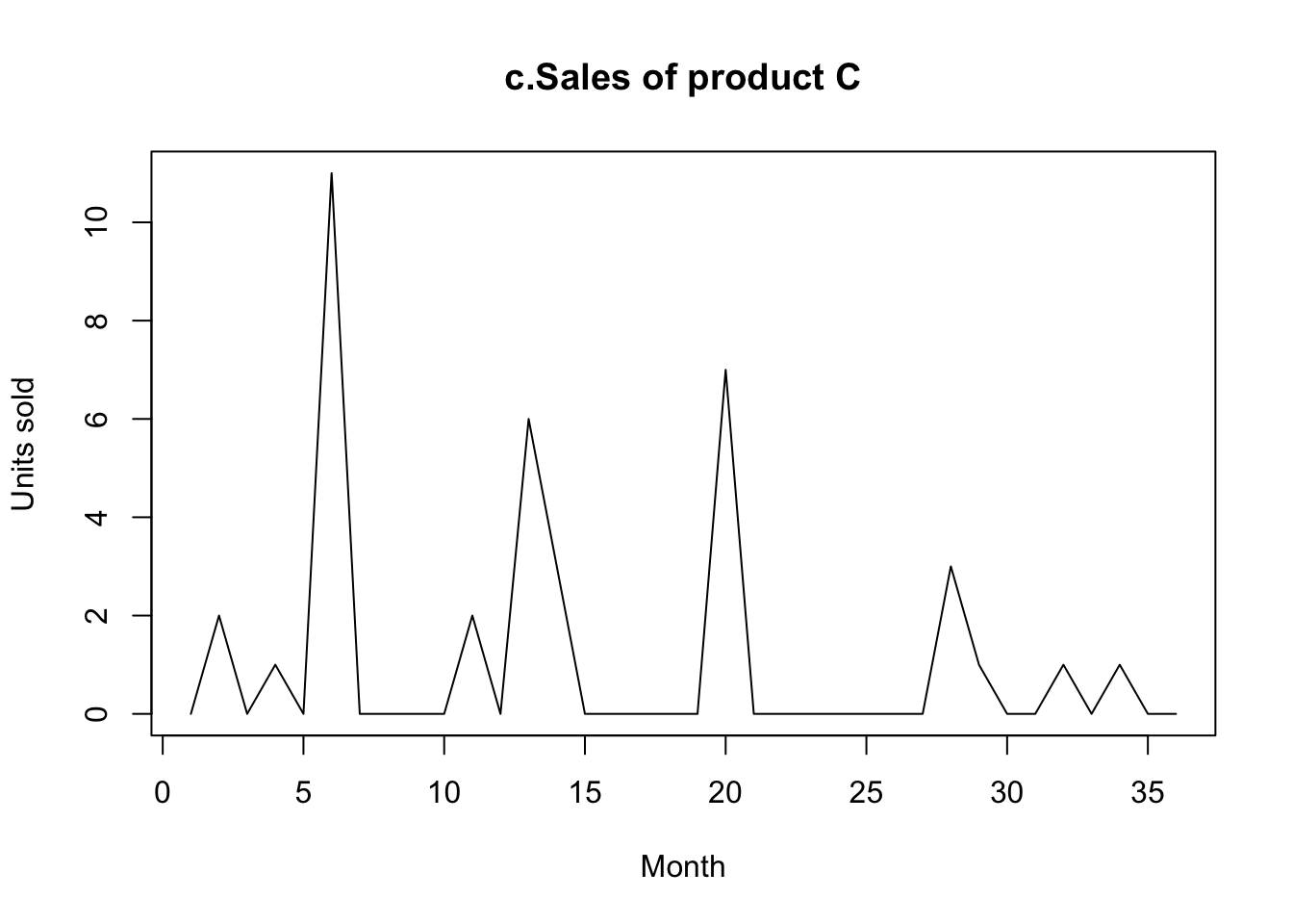
plot(ts(ProductC),ylab="Units sold",xlab="Month",main="c.Sales of product C")
 
################################################
 
Brick <- c(
  189, 204, 208, 197, 187, 214, 227, 223, 199, 229,
  249, 234, 208, 253, 267, 255, 242, 268, 290, 277,
  241, 253, 265, 236, 229, 265, 275, 258, 231, 263,
  308, 313, 293, 328, 349, 340, 309, 349, 366, 340,
  302, 350, 362, 337, 326, 358, 359, 357, 341, 380,
  404, 409, 383, 417, 454, 428, 386, 428, 434, 417,
  385, 433, 453, 436, 399, 461, 476, 477, 452, 461,
  534, 516, 478, 526, 518, 417, 340, 437, 459, 449,
  424, 501, 540, 533, 457, 513, 522, 478, 421, 487,
  470, 482, 458, 526, 573, 563, 513, 551, 589, 564,
  519, 581, 581, 578, 500, 560, 512, 412, 303, 409,
  420, 413, 400, 469, 482, 484, 447, 507, 533, 503,
  443, 503, 505, 443, 415, 485, 495, 458, 427, 519,
  555, 539, 511, 572, 570, 526, 472, 524, 497, 460,
  373, 436, 424, 430, 387, 413, 451, 420, 394, 462,
  476, 443, 421, 472, 494
)
 
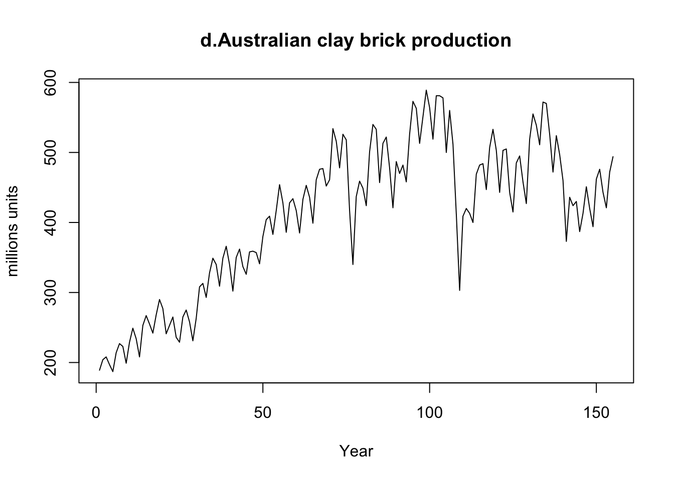
plot(ts(Brick),ylab="millions units",xlab="Year",main="d.Australian clay brick production")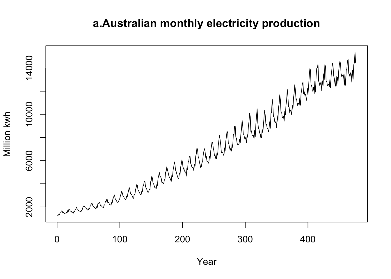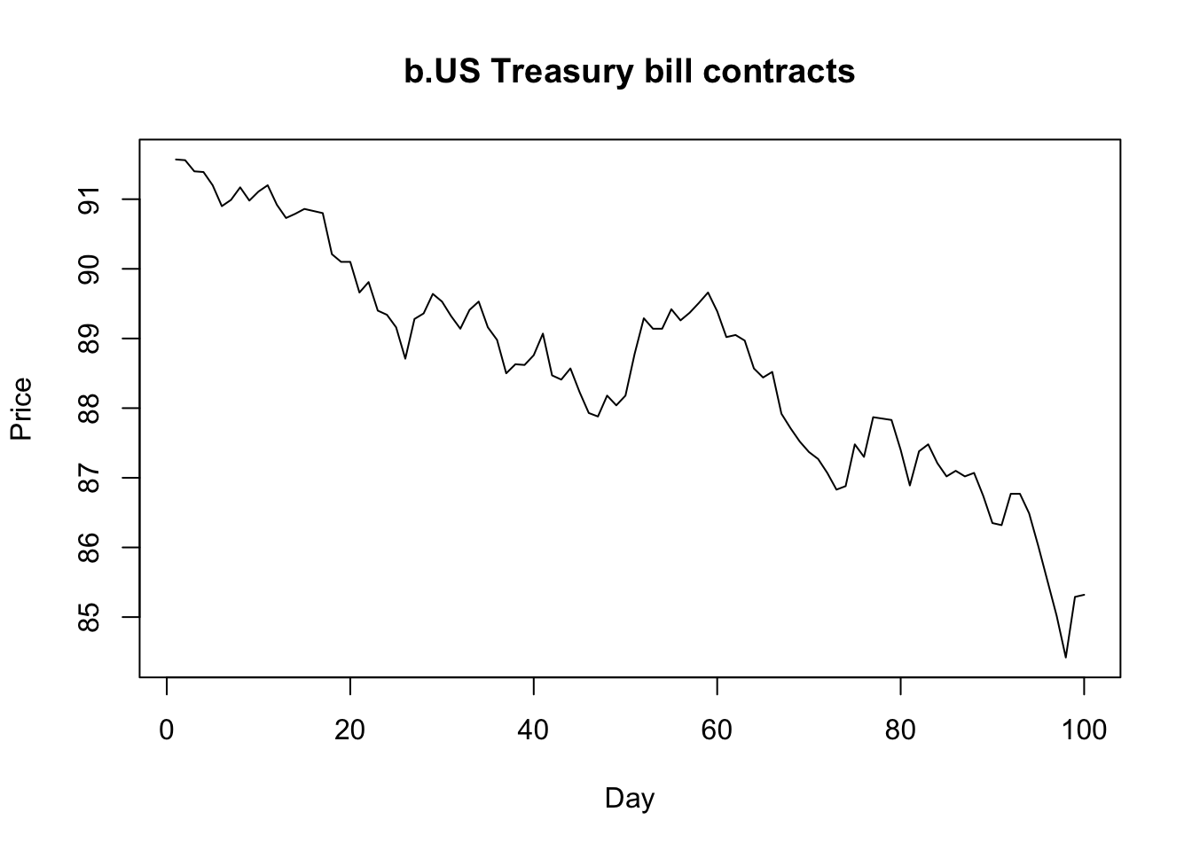

a. We see an increasing trend over time in the time series. There is also seasonal behaviour present in the data. Over time we see an increase in the variation of the time series. This pattern is often referred to as multiplicative seasonality.
b. This time series only shows a decreasing trend over time.

c. This time series is relatively constant around zero, with a few spikes.
d. This time series starts with an increasing trend, then becomes almost constant over time. This time series contains seasonal behaviour and well as a cyclical pattern. The seasonal pattern is visible within each cycle. Seasonality is a constant behaviour in fixed time periods (e.g., quarterly, or yearly). A cycle is not constant and takes place over larger periods.

Chapter 2: Basic Forecasting Tools

Time series and cross-sectional data

The Cars data contains 45 observations and two variables Mileage (X) and Price (Y). Since the Price of the car is dependent on the Mileage, we can use it to predict the Price. This dataset is considered a cross-sectional dataset, which is a set of measurement taken at a point in time.
The Australian beer data contains 56 observations of the beer production. Note that this is typically what a time series looks like, which contains a set of measurements over time. There is a time unit part of the data (months and years) hence the name time series. Other units often used to represent a time series are hours, days, or weeks.

#| label: Aussie beer
library(readxl)
Beer <- read_excel("~/Documents/DataEng/5thYear/Semester 2/Stats 348/Part B/Datasets/Australian beer data.xlsx")
head(Beer)

{#output-Aussie beer}

New names:
# A tibble: 6 x 4
  `1...1` `1991` `1...3` `164`
    <dbl>  <dbl>   <dbl> <dbl>
1       2   1991       2   148
2       3   1991       3   152
3       4   1991       4   144
4       5   1991       5   155
5       6   1991       6   125
6       7   1991       7   153

Graphical summaries

Time plots and time series patterns

#| label: Time series plot
years <- unique(Beer[,2])[[1]]
plot(Beer[,c(1,4)],type="l",xaxt="n",ylab="MegaLiters",xlab="Year",main="Monthly Australian beer production")
axis(side = 1, at = c(1, 13, 25, 37, 49), labels = years)

The time series do not seem to have any trend (upward or downward) and varies around a constant. However, we see a seasonal behaviour over time. At every 12th month there is a huge spike/ increase in the number of Liters produced. This is typical of seasonal behaviour. In this case it happens at the end of each year, thus yearly seasonality is present in the production of the beer.

A ==horizontal (H)== pattern exists when the time series fluctuate horizontal around a constant mean. (Such a series is called stationary in its mean.) A product whose sales do not increase or decrease over time would be of this type.
A ==seasonal (S)== pattern exists when a series is influenced by seasonal factors (e.g., the quarter of the year, the month, or day of the week). Sales of products such as soft drinks, ice creams, and household electricity consumption all exhibit this type of pattern. The beer data show seasonality with a peak in production in November and December (in preparation for Christmas) each year.
A ==cyclical (C)== pattern exists when the data exhibit rises and cyclical falls that are not of a fixed period.
A ==trend (T)== pattern exists when there is a long-term increase or trend decrease in the data. The sales of many companies, the gross national product (GNP), and many other business or economic indicators follow a trend pattern in their movement over time. The electricity production data shown in Assignment 1-1.png exhibit a strong trend in addition to the monthly seasonality. The beer data in Time series plot-1.png shows no trend.
An ==irregular (random) (E)== component usually exist if there are no other identifiable pattern.

In Chapter 3 Time Series Decomposition we will use the symbols T, S, C and E in our discussion of decomposition methods.

Seasonal plots

#| label: Seasonal Plot
months <- c("Jan","Feb","Mar","Apr","May","Jun","July","Aug","Sep","Oct","Nov","Dec")
plot(Beer[1:12,c(3,4)],ylab="MegaLiters",xlab="Months", xaxt="n", main="Monthly Australian beer production",type="l",col="red")
points(Beer[13:24,c(3,4)],col="blue",type="l")
points(Beer[25:36,c(3,4)],col="black",type="l")
points(Beer[37:48,c(3,4)],col="green",type="l")
points(Beer[49:56,c(3,4)],col="orange",type="l")
axis(side=1,at=c(1,2,3,4,5,6,7,8,9,10,11,12),labels=months)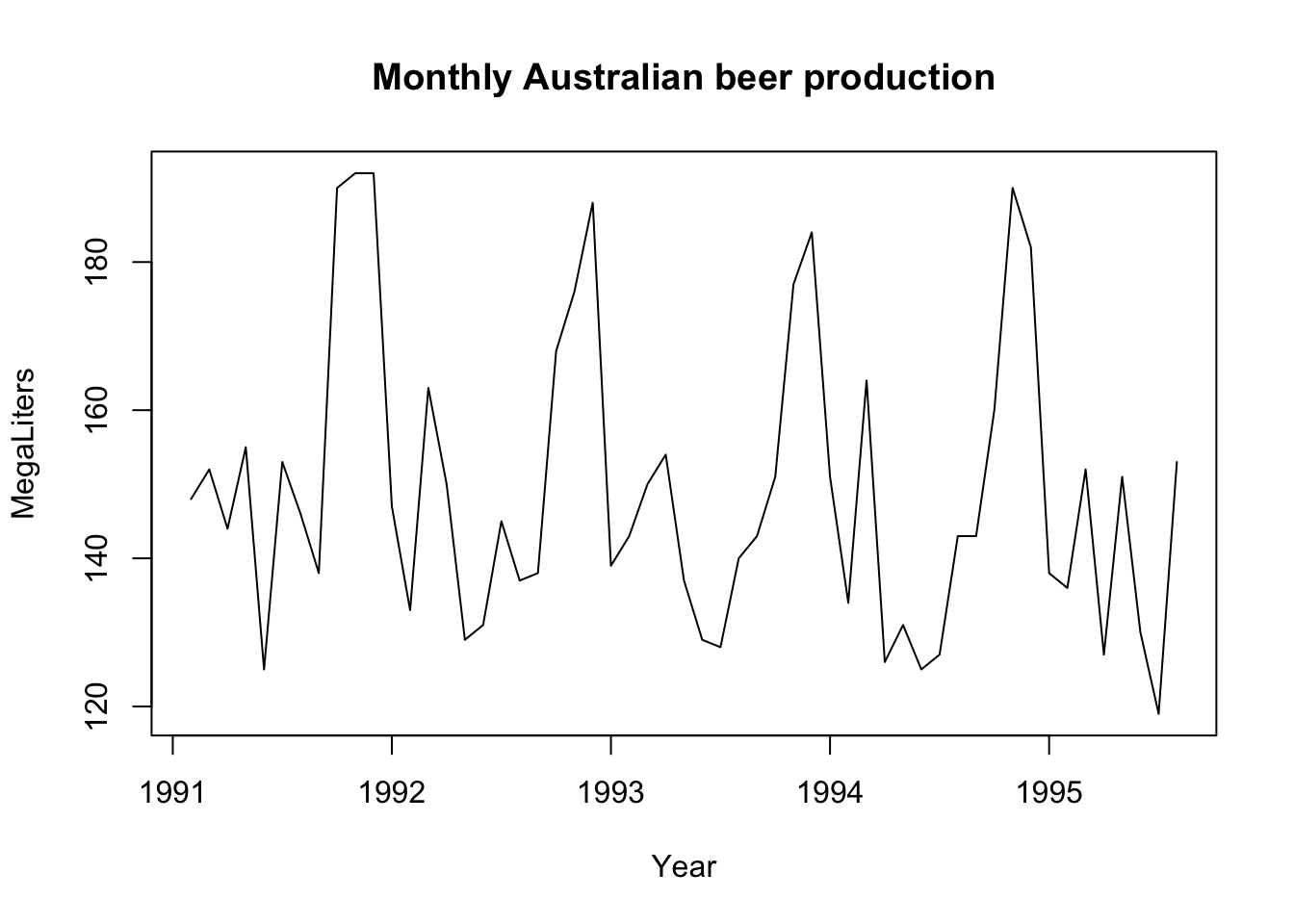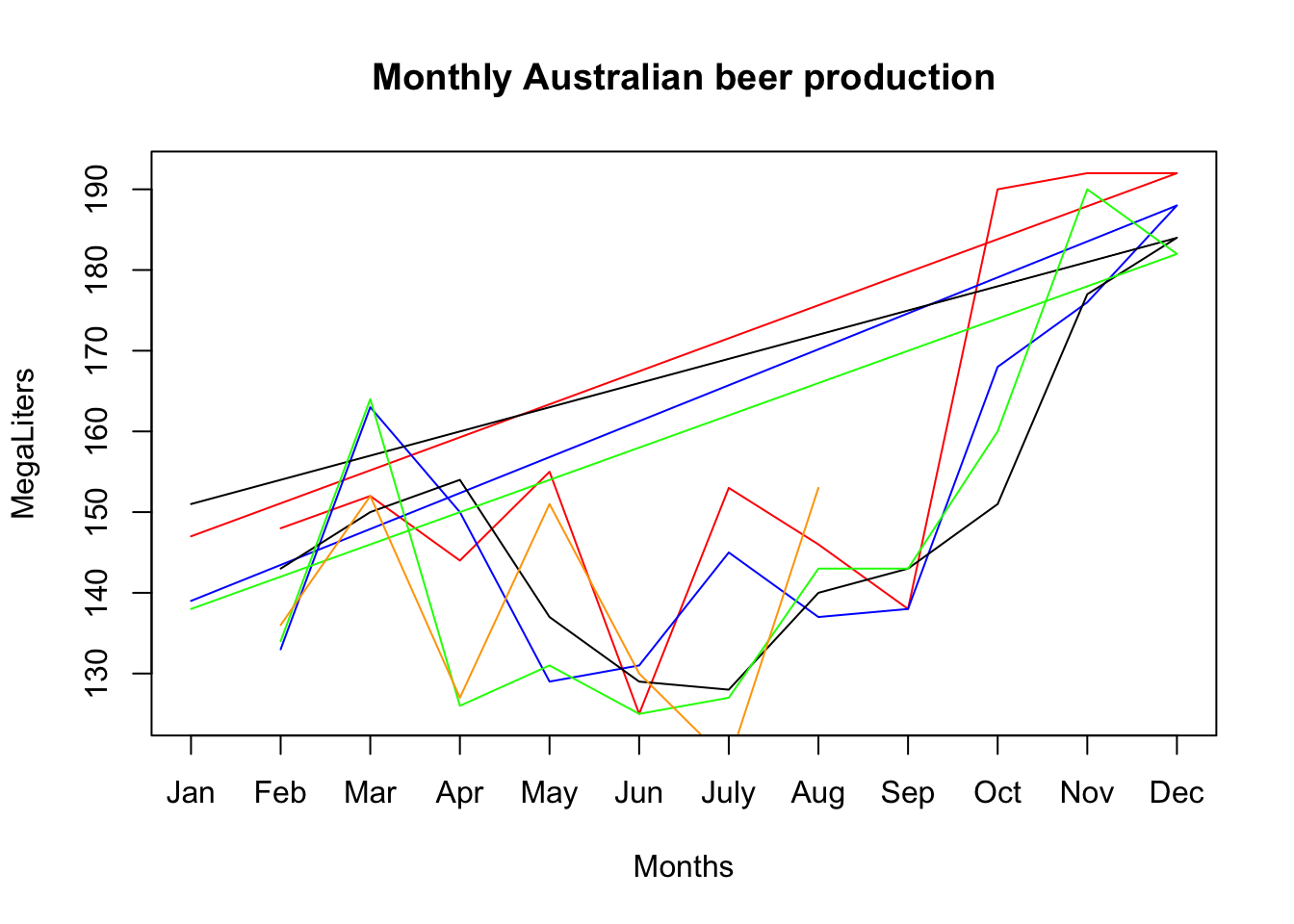

Scatterplots

#| label: Cars data
#Cars <- read.table(pipe("pbpaste"))
library(readxl)
Cars <- read_excel("~/Documents/DataEng/5thYear/Semester 2/Stats 348/Part B/Datasets/Cars data.xlsx")
Cars <- Cars[,2:4]
head(Cars)
#str(Cars)
Japan<-Cars[Cars[,1]=="Japan",]
USA<-Cars[Cars[,1]=="USA",]

{#output-Cars data}

New names:
# A tibble: 6 x 3
  Country Milage Price
  <chr>    <dbl> <dbl>
1 Japan       19 14944
2 Japan       19 14799
3 Japan       20 24760
4 Japan       20 14929
5 Japan       20 13949
6 Japan       21 17879

#| label: Scatterplots
plot(Cars$Milage, Cars$Price,xlab = "Mileage (mpg)",ylab = "Price",main = "Price/Mileage relationship of 45 automobiles")
plot(Japan[,c(2,3)],pch=1,col="red",ylab="Price",xlab="Mileage(mpg)",main="Price/Mileage relationship of 45 automobiles")
 
points(USA[,c(2,3)],pch=2,col="blue")
 
legend(28,23000,col=c("red","blue"),pch=c(1,2),c("Made in Japan","Made in USA"))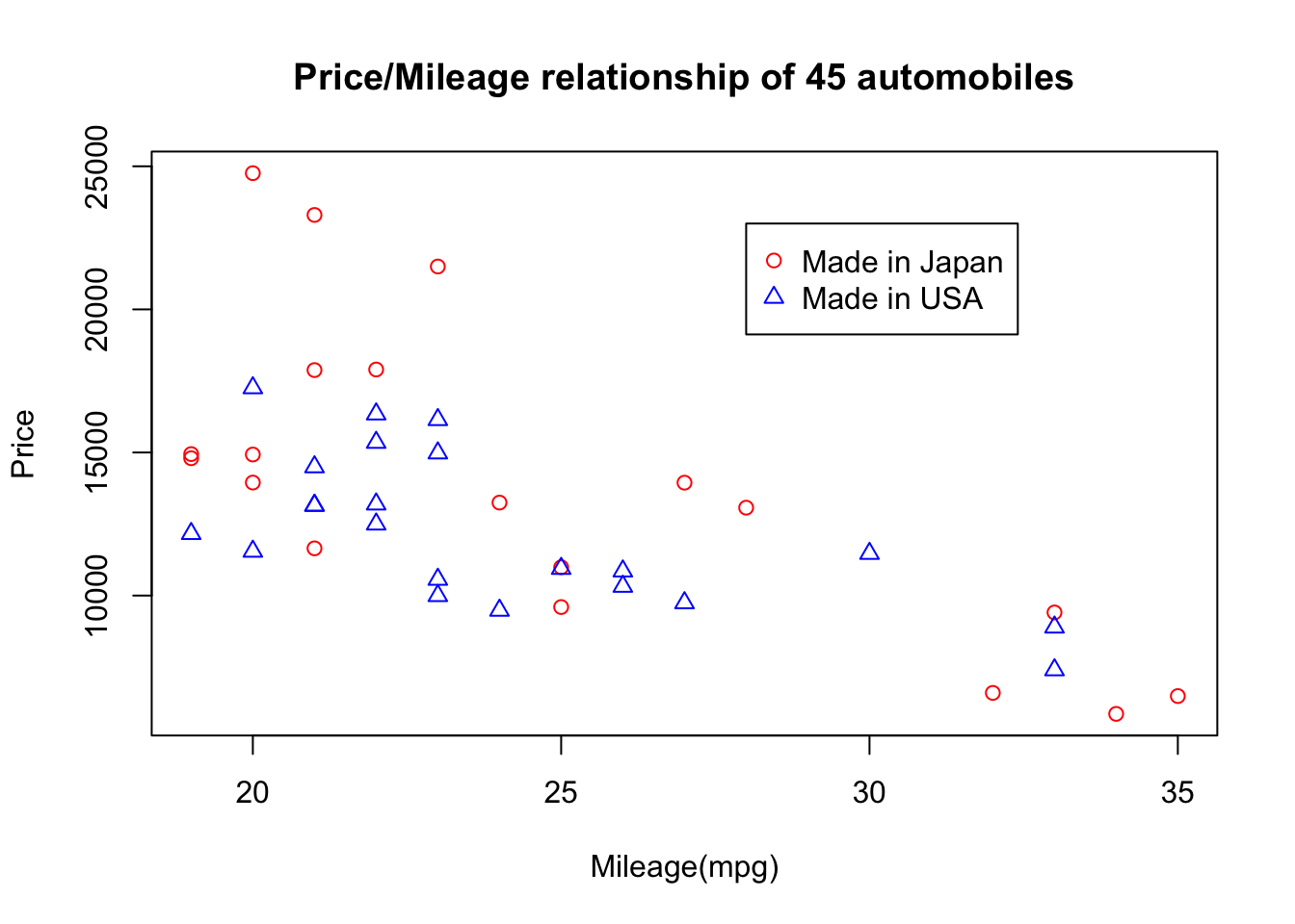

Numerical summaries

Univariate Statistics

Mean

\overset{ˉ}{Y} = \frac{1}{n} \sum Y_{i} (2.1)

Median (middle value)

M e d ian = x_{(\frac{n + 1}{2})} (2.2)

if n is odd:
	Median is the middle value

if n is even:
	Median is the average of the 2 middle values

MAD (Mean Absolute Deviation)

M A D = \frac{1}{n} \sum ∣ Y_{i} - \overset{ˉ}{Y} ∣ (2.3)

MSD (Mean Squared Deviation

MS D = \frac{1}{n} \sum (Y_{i} - \overset{ˉ}{Y})^{2} (2.4)

Variance

S^{2} = \frac{1}{n - 1} \sum (Y_{i} - \overset{ˉ}{Y})^{2} (2.5)

Standard Deviation

S = S^{2} = \frac{1}{n - 1} \sum (Y_{i} - \overset{ˉ}{Y})^{2} (2.6)

#| label: univariate
Y<-Japan$Milage
 
# mean
Ybar <- mean(Y)
Ybar
 
# median
Med <- median(Y)
Med
 
# MAD
MAD <- mad(Y)
MAD
 
# MSD
MSD <- mean((Y-Ybar)^2)
MSD
 
# Var
var <- var(Y)
var
 
# sd 
sd <- sd(Y)
sd

{#output-univariate}

[1] 24.68421

[1] 23

[1] 4.4478

[1] 27.05817

[1] 28.5614

[1] 5.344287

Bivariate Statistics

#| label: bivariate
 
# covariance
var(Japan[,c(2,3)])
 
# correlation
cor(Japan[,c(2,3)])

{#output-bivariate}

Milage       Price
Milage     28.5614   -21001.54
Price  -21001.5380 29160066.83

           Milage      Price
Milage  1.0000000 -0.7277246
Price  -0.7277246  1.0000000

There appears to be a strong negative relationship between Mileage and Price for the Cars data. If the Mileage is high, the Price is lower. This confirms what was displayed in the graphs.

Autocorrelation

Autocovariance

c_{k} = \frac{1}{n} t = k + 1 \sum n (Y_{t} - \overset{ˉ}{Y}) (Y_{t - k} - \overset{ˉ}{Y}) (2.10)

Autocorrelation

r_{k} = \frac{\sum _{t = k + 1}^{n} ( Y _{t} - Y ˉ ) ( Y _{t - k} - Y ˉ )}{\sum _{t = 1}^{n} ( Y _{t} - Y ˉ ) ^{2}} (2.11)

$Y_{t}$ is the observation at time t. The observation $Y_{t - 1}$ refers to the observation at time $t - 1$ and similarly for $t - 2, \dots, t - k$
Observation $Y_{t - 1}$ is described as “lagged” by one period
If $k = 1$ , then the sample auto-covariance and autocorrelation for one lag is:

c_{1} = \frac{1}{n} t = 1 + 1 = 2 \sum n (Y_{t} - \overset{ˉ}{Y}) (Y_{t - 1} - \overset{ˉ}{Y}) (2.10)

r_{1} = \frac{\sum _{t = 1 + 1 = 2}^{n} ( Y _{t} - Y ˉ ) ( Y _{t - 1} - Y ˉ )}{\sum _{t = 1}^{n} ( Y _{t} - Y ˉ ) ^{2}} (2.11)

This autocorrelation tells us whether there is a correlation between $Y_{t}$ and $Y_{t - 1}$ .

Similarly for $k = 2$ and so on.
Often we calculate these autocorrelations for different lags. Together, the autocorrelations $r_{1}, r_{2}, \dots, r_{k}$ form the autocorrelation function (ACF).
Plotting these autocorrelations are referred to as a correlogram or an ACF plot. We can easily obtain the autocovariance, autocorrelation and their respective ACF plots using R.
The following commands were used to obtain the autocovariances for 20 lags using the

Australian beer data:

#| label: acf 
cov_afc <- acf(Beer[,4],lag.max=20,type="covariance")
cor_afc <-acf(Beer[,4],lag.max=20,type="correlation")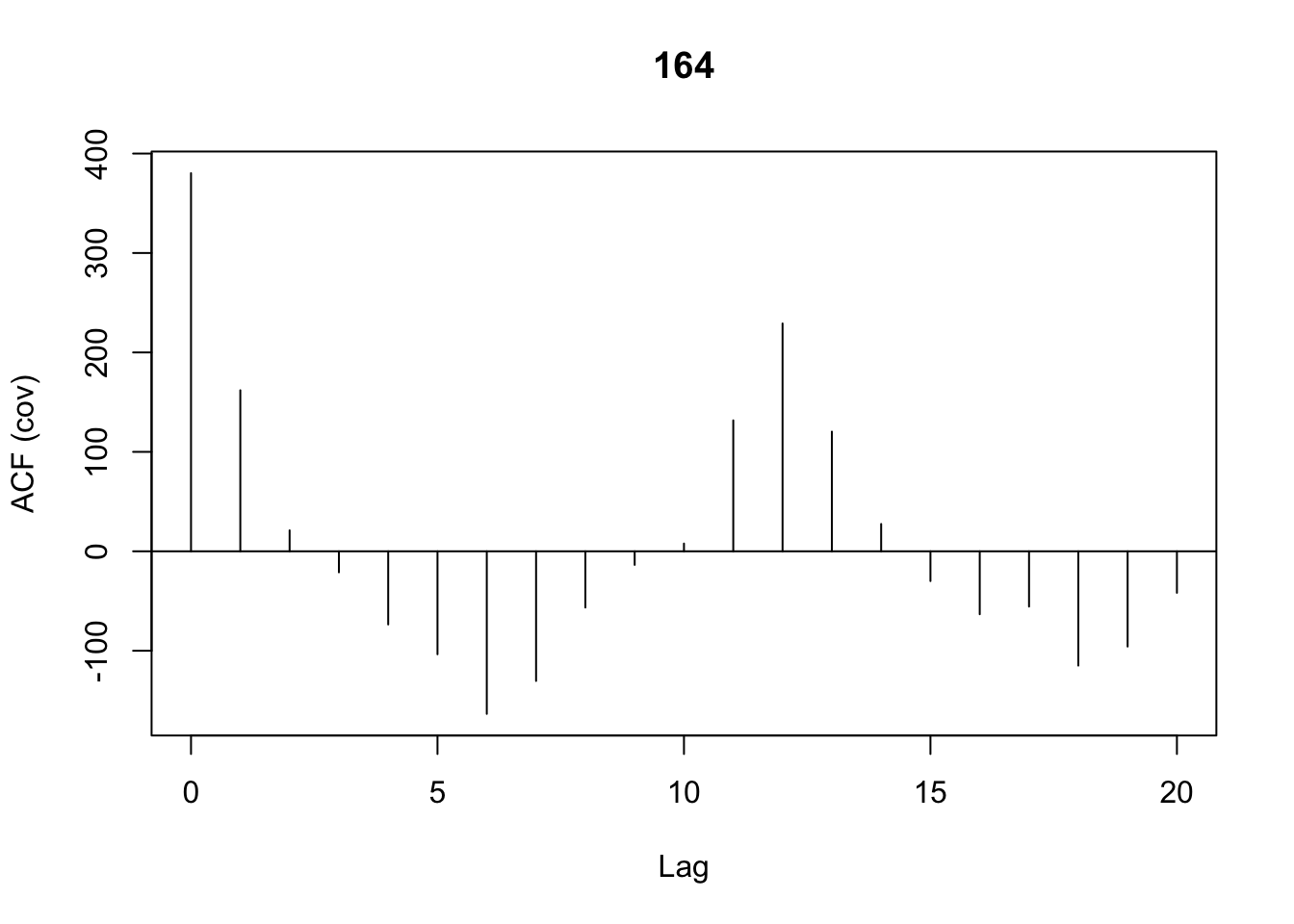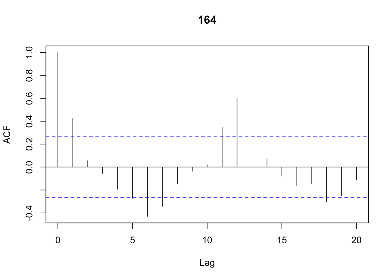

The blue dotted lines ( $- - -$ ) are called the ACF critical values. These lines are obtained using $2/ n$ . Notice the centre is zero, thus the interval is $\pm 2/ n$ . For the Australian beer data $n = 56$ , giving us an interval of $\pm 2/ 56 = \pm 0.267$ .

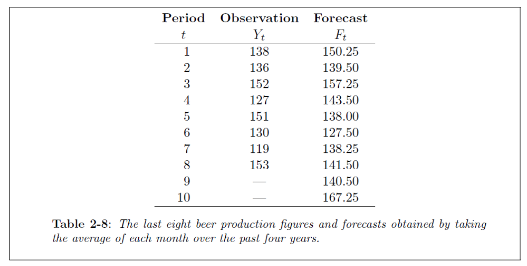
Measuring forecast accuracy

Consider this Table, containing a time series (Y) for $n = 8$ observations. These observations are the 1995 cases (January to August). The forecasts (F) for this example are the average over the other years 1991-1994 for each month.

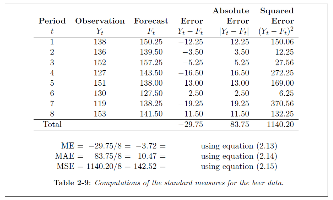
Standard statistical measures

ME = Mean Error

ME = \frac{1}{n} t = 1 \sum n (Y_{t} - F_{t})

MAE = Mean Absolute Error

M A E = \frac{1}{n} t = 1 \sum n ∣ Y_{t} - F_{t} ∣

MSE = Mean Square Error

MSE = \frac{1}{n} t = 1 \sum n (Y_{t} - F_{t})^{2}

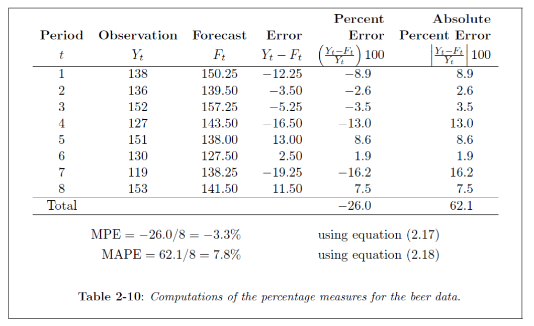
PE = Percentage Error

P E_{t} = [\frac{Y _{t} - F _{t}}{Y _{t}}] \times 100

MPE = Mean Percentage Error

MPE = \frac{1}{n} t = 1 \sum n P E_{t}

MAPE = Mean Absolute Percentage Error

MPE = \frac{1}{n} t = 1 \sum n ∣ P E_{t} ∣

In these measures, $Y_{t}$ refers to the time series observation and $F_{t}$ the forecast at time $t$ .
Thus, $Y_{t + 1}$ and $F_{t + 1}$ refers to similar values at time $t + 1$ (one period into the future).

This Table shows the calculation of the ME, MAE and MSE. The MSE is often the popular choice to assess the forecasting method.

Out-of-sample accuracy measurement

The summary statistics discussed so far measures the goodness-of-fit of the model on historical data (training data). The drawback of the measures based on the training data is that tend to be biased and will show a good fit.
To overcome this problem, we often split the training data into a “initialization set” and a “test set”. The model is fitted on the initialization set and the goodness-of-fit measures are calculated on the test set.

Comparing forecast methods

Theil's U-statistic

ACF of forecast error

#| label: errors
 
# Extract Y = 1995 values (first 8 months)
Y <- Beer[Beer[[2]] == 1995, ][[4]][1:8]
 
# Extract F = mean of other years, grouped by month (col 1)
F <- tapply(
  Beer[Beer[[2]] != 1995, ][[4]],  # production values
  Beer[Beer[[2]] != 1995, ][[3]],  # group by month
  mean
)[1:8]
 
Y
F 
 
e = Y - F 
e

{#output-errors}

[1] 138 136 152 127 151 130 119 153

       1        2        3        4        5        6        7        8 
145.6667 139.5000 157.2500 143.5000 138.0000 127.5000 138.2500 141.5000 

         1          2          3          4          5          6          7 
 -7.666667  -3.500000  -5.250000 -16.500000  13.000000   2.500000 -19.250000 
         8 
 11.500000

#| label: acf_errors
cor_afc <-acf(e,type="correlation")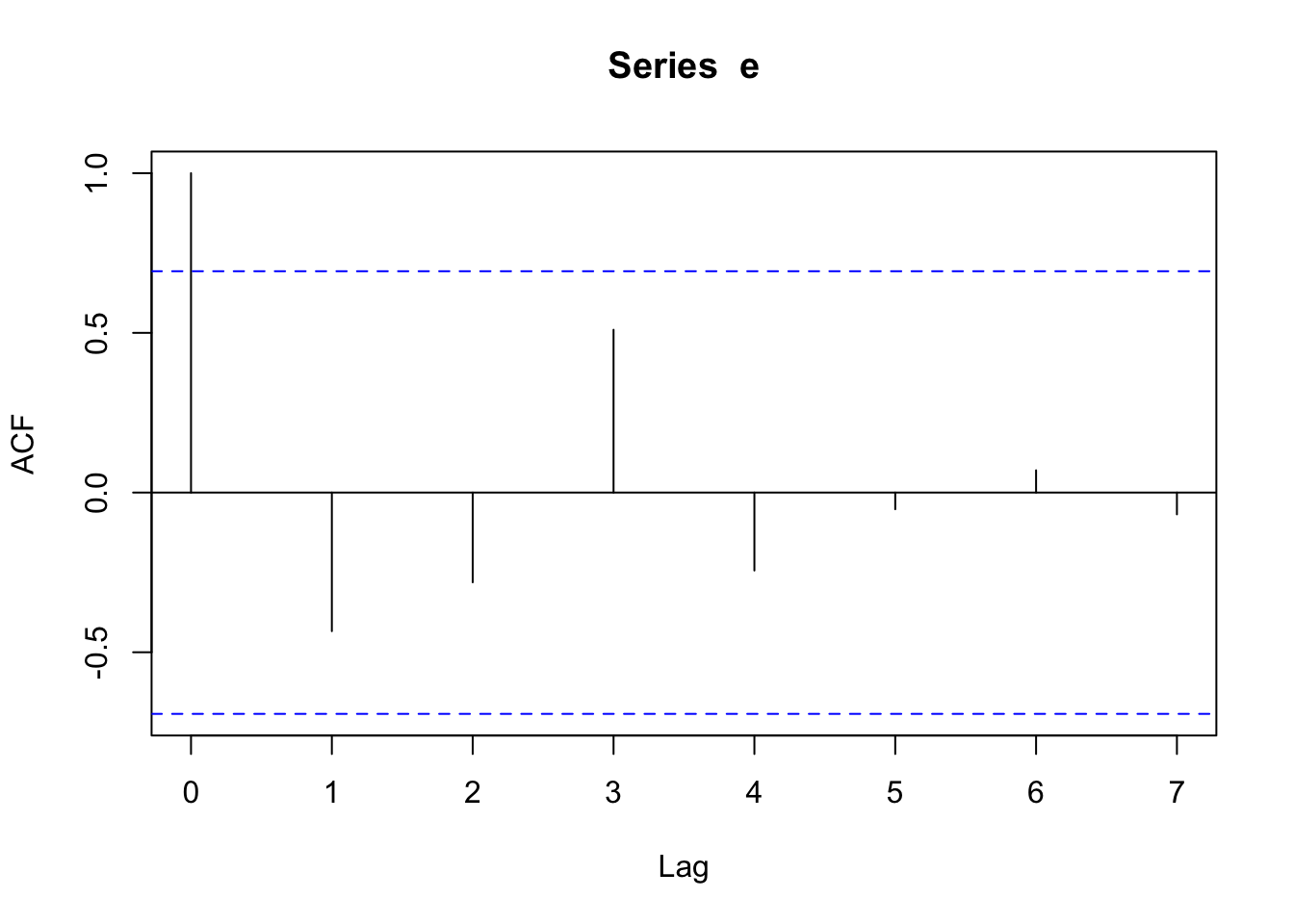

Prediction intervals

Least squares estimates

Example 1

Consider the Error Sum of Squares (SSE):

SSE = i = 1 \sum n (Y_{i} - \hat{Y_{i}})^{2}

Let $\hat{Y_{i}} = a$ , which is a constant. Show that the value (constant) that will minimize the SSE is the sample mean ( $\overset{ˉ}{Y}$ ).

Proof: Write the SSE as

SSE = i = 1 \sum n (Y_{i} - a)^{2} = i = 1 \sum n (Y_{i}^{2} - 2 a Y_{i} + a^{2}) = i = 1 \sum n Y_{i}^{2} - 2 a i = 1 \sum n Y_{i} + n a^{2}

Taking the derivative w.r.t $a$ and putting it equal to zero, leads to the following result:

\frac{d SSE}{d a} = - 2 i = 1 \sum n Y_{i} + 2 na na a = 0 = i = 1 \sum n Y_{i} = \frac{1}{n} i = 1 \sum n Y_{i} = \overset{ˉ}{Y}

Thus, the mean ( $\overset{ˉ}{Y}$ ) will minimize the SSE.

Example 2

Consider again the Error Sum of Squares (SSE):

SSE = i = 1 \sum n (Y_{i} - \hat{Y_{i}})^{2}

Now, let $\hat{Y_{i}} = a + b X_{i}$ , which is a linear function. Show that the values (constants) $a$ and $b$ that will minimize the SSE are $a = \overset{ˉ}{Y} - b \overset{ˉ}{X}$ and $b = \frac{\sum _{i = 1}^{n} ( X _{i} - X ˉ ) ( Y _{i} - Y ˉ )}{\sum _{i = 1}^{n} ( X _{i} - X ˉ ) ^{2}}$ .

Proof: Write the SSE as

SSE = i = 1 \sum n (Y_{i} - \hat{Y_{i}})^{2} = i = 1 \sum n [Y_{i}^{2} - 2 Y_{i} \hat{Y_{i}} + \hat{Y_{i}}^{2}] = i = 1 \sum n Y_{i}^{2} - 2 i = 1 \sum n Y_{i} \hat{Y_{i}} + i = 1 \sum n \hat{Y_{i}}^{2} = i = 1 \sum n Y_{i}^{2} - 2 i = 1 \sum n Y_{i} (a + b X_{i}) + i = 1 \sum n (a + b X_{i})^{2} = i = 1 \sum n Y_{i}^{2} - 2 i = 1 \sum n (a Y_{i} + b X_{i} Y_{i}) + i = 1 \sum n (a^{2} + 2 ab X_{i} + b^{2} X_{i}^{2}) = i = 1 \sum n Y_{i}^{2} - 2 a i = 1 \sum n Y_{i} - 2 b i = 1 \sum n X_{i} Y_{i} + n a^{2} + 2 ab i = 1 \sum n X_{i} + b^{2} i = 1 \sum n X_{i}^{2}

Taking the derivative w.r.t $a$ and $b$ , and putting it equal to zero, leads to the following result:

\frac{\partial SSE}{\partial a} = - 2 i = 1 \sum n Y_{i} + 2 na + 2 b i = 1 \sum n X_{i} - 2 \overset{ˉ}{Y} + 2 a + 2 b \overset{ˉ}{X} - \overset{ˉ}{Y} + a + b \overset{ˉ}{X} ∴ \overset{ˉ}{Y} = 0 = 0 = 0 = a + b \overset{ˉ}{X}

\frac{\partial SSE}{\partial b} = - 2 i = 1 \sum n X_{i} Y_{i} + 2 a i = 1 \sum n X_{i} + 2 b i = 1 \sum n X_{i}^{2} - i = 1 \sum n X_{i} Y_{i} + a i = 1 \sum n X_{i} + b i = 1 \sum n X_{i}^{2} = 0 = 0

Using result $\overset{ˉ}{Y} = a + b \overset{ˉ}{X}$ , we rewrite to $a = \overset{ˉ}{Y} - b \overset{ˉ}{X}$

- i = 1 \sum n X_{i} Y_{i} + (\overset{ˉ}{Y} - b \overset{ˉ}{X}) i = 1 \sum n X_{i} + b i = 1 \sum n X_{i}^{2} - i = 1 \sum n X_{i} Y_{i} + \overset{ˉ}{Y} i = 1 \sum n X_{i} - b \overset{ˉ}{X} i = 1 \sum n X_{i} + b i = 1 \sum n X_{i}^{2} b [i = 1 \sum n X_{i}^{2} - \overset{ˉ}{X} i = 1 \sum n X_{i}] = 0 = 0 = i = 1 \sum n X_{i} Y_{i} - \overset{ˉ}{Y} i = 1 \sum n X_{i}

∴ b = \frac{\sum _{i = 1}^{n} X _{i} Y _{i} - Y ˉ \sum _{i = 1}^{n} X _{i}}{\sum _{i = 1}^{n} X _{i}^{2} - X ˉ \sum _{i = 1}^{n} X _{i}}

With some algebraic manipulation, we get

b = \frac{\sum _{i = 1}^{n} ( X _{i} - X ˉ ) ( Y _{i} - Y ˉ )}{\sum _{i = 1}^{n} ( X _{i} - X ˉ ) ^{2}} = \frac{co v ( X , Y )}{v a r ( X )}

Transformations and adjustments

Transformations of the raw time series is often needed, which may lead to a simpler and more interpretable choice the forecasting model.

Mathematical transformations

A few standard transformations for stabilizing the variation in a time series:

Square root: $W_{t} = Y_{t}$
Cube root: $W_{t} = 3 Y_{t}$
Logarithm: $W_{t} = l o g (Y_{t})$
Negative reciprocal: $W_{t} = - 1/ Y_{t}$

Calendar adjustments

In forecasting related to business data, often we may need to adjust the time series using for example month length adjustments or trading day adjustments.

Adjustments for inflation and population changes

In forecasting related to government data, we may need to adjust the time series for the effect of inflation or for changes in the population.

Chapter 3: Time Series Decomposition

Principles of decomposition

Decomposition models

In general, we use the mathematical model

Y_{t} = f (S_{t}, T_{t}, E_{t}), t = 1, \dots, n

The exact form depends on the decomposition method used.

The additive decomposition model has the mathematical form

Y_{t} = S_{t} + T_{t} + E_{t}

The multiplicative decomposition model has the mathematical form

Y_{t} = S_{t} \times T_{t} \times E_{t}

By taking the logarithm of the multiplicative model, we get

l o g (Y_{t}) = l o g (S_{t}) + l o g (T_{t}) + l o g (E_{t})

which is an additive decomposition in log form.

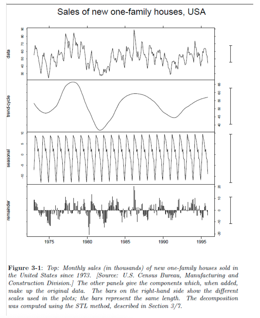
Decomposition graphics

The top graph is just a time series plot of the data
The second graph is the Trend- Cycle plot (in Moving Averages (MA) we will discuss “moving averages” and in Local Regression Smoothing we will discuss “moving lines”)
The third graph is the Seasonality plot and
The bottom graph is the Error ACF Plot (or often called the remainder).

Moving Averages (MA)

The purpose of the moving average is to estimate the Trend-Cycle component from the time series. In a sense we are smoothing the time series.

Simple moving averages

The formula for the simple moving average of order k (or k MA) can be defined as:

T_{t} = \frac{1}{k} j = - m \sum m Y_{t + j} = \frac{1}{k} [Y_{t - m} + Y_{t - (m - 1)} + \dots + Y_{t} + Y_{t + (m - 1)} + Y_{t + m}]

where, $T_{t}$ is the Trend-Cycle estimate at time $t$ , with $k$ being any odd number and $m = \frac{k - 1}{2}$ .

Consider the formula for $k = 5$ , thus $m = \frac{k - 1}{2} = \frac{5 - 1}{2} = 2$ and

T_{t} = \frac{1}{5} [Y_{t - 2} + Y_{t - 1} + Y_{t} + Y_{t + 1} + Y_{t + 2}] = \frac{1}{5} Y_{t - 2} + \frac{1}{5} Y_{t - 1} + \frac{1}{5} Y_{t} + \frac{1}{5} Y_{t + 1} + \frac{1}{5} Y_{t + 2}

From this we notice that there are five observations, each with the same weight $[\frac{1}{5}; \frac{1}{5}; \frac{1}{5}; \frac{1}{5}; \frac{1}{5}]$ .

Thus, each observation in the time series is weighted equally.
Using the Shampoo data.xlsx we can construct the k MA for $k = 3$ and $k = 5$ using the following R commands.

#| label: kMA
library(readxl)
Shampoo <- read_excel("~/Documents/DataEng/5thYear/Semester 2/Stats 348/Part B/Datasets/Shampoo data.xlsx")
 
Y<-ts(Shampoo,freq=3)
MA3<-decompose(Y)$trend
plot(Y, ylab="Amount",xlab="Months", main="3MA smoother")
lines(MA3,lty=2,col="red")
 
Y<-ts(Shampoo,freq=5)
MA5<-decompose(Y)$trend
plot(Y, ylab="Amount",xlab="Months", main="5MA smoother")
lines(MA5,lty=3,col="blue")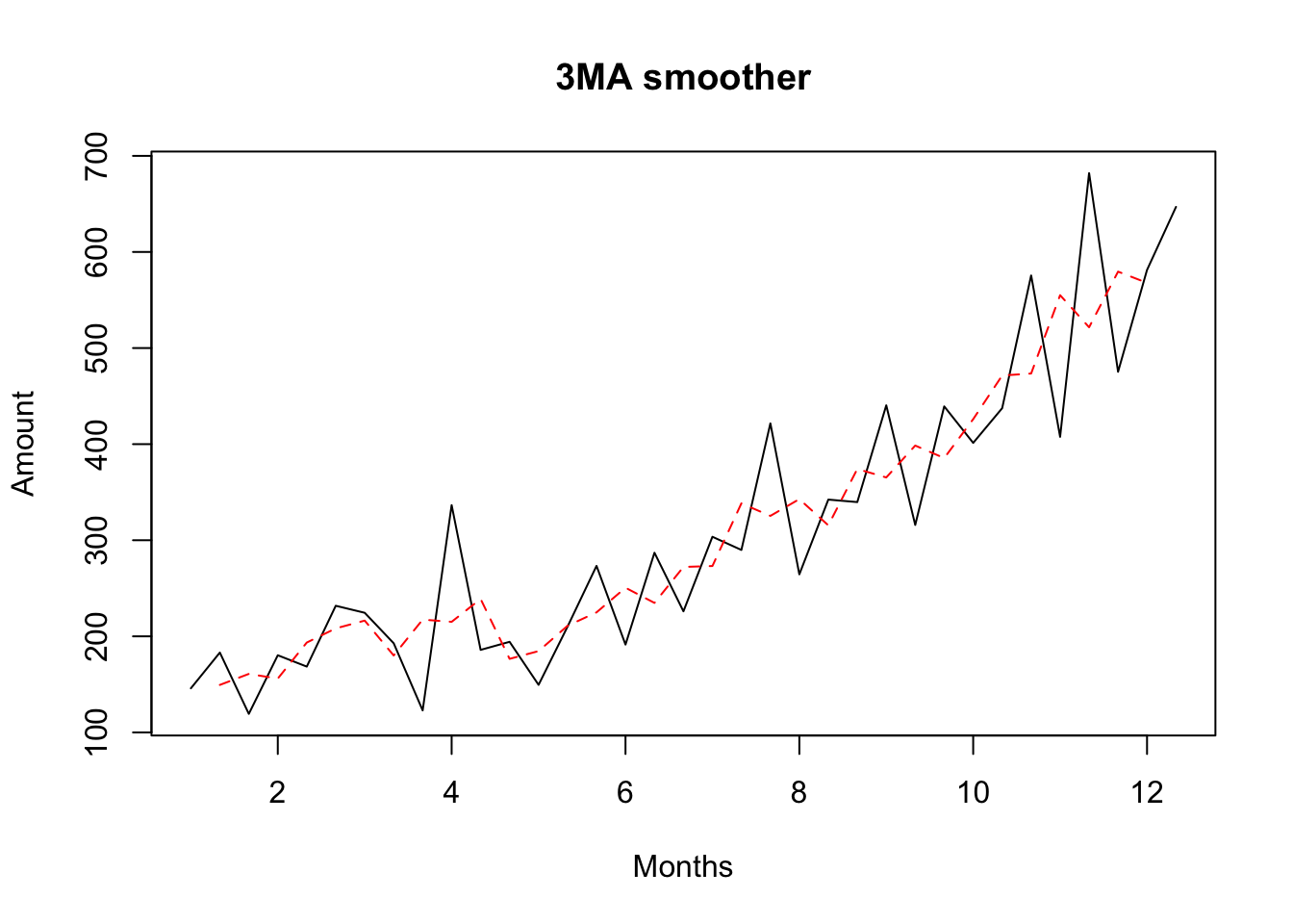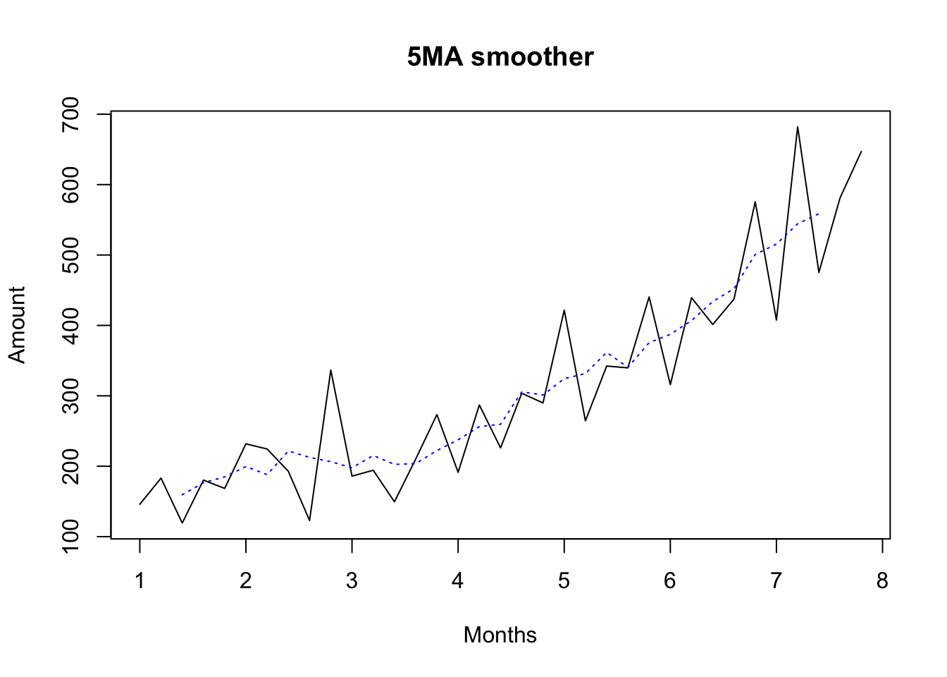

3MA vs 5MA smoothers for the shampoo data. The 3MA smoother leaves too much randomness in the trend-cycle estimate. The 5MA smoother is better, but the true trend-cycle is probably smoother still.

Centered moving averages

Centered moving averages works with even numbers.
Consider the table. The 4 MA column contains the moving average of 4 cases. The column 2x4 MA contains the moving average of 2 cases from the column of the 4 MA.

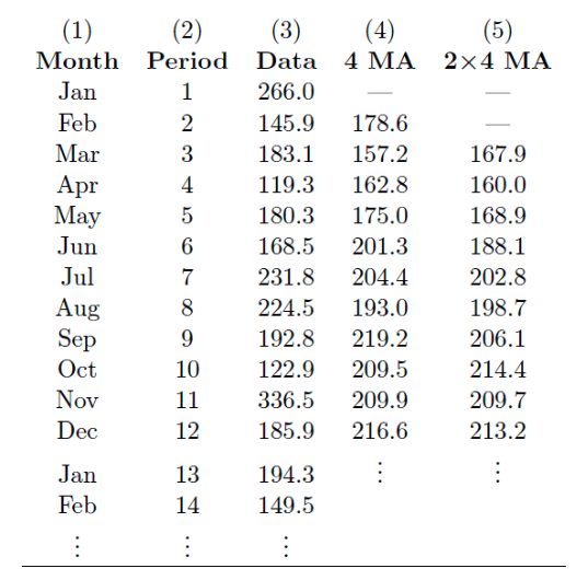
Examples of the 4 MA:

T_{2.5} = \frac{1}{4} (Y_{1} + Y_{2} + Y_{3} + Y_{4}) = \frac{1}{4} (266 + 145.9 + 183.1 + 119.3) = 178.6

T_{3.5} = \frac{1}{4} (Y_{2} + Y_{3} + Y_{4} + Y_{5}) = \frac{1}{4} (145.9 + 183.1 + 119.3 + 180.3) = 157.2

Examples of the 2x4 MA:

\frac{1}{2} (T_{2.5} + T_{3.5}) = \frac{1}{2} (178.6 + 157.2) = 167.9

Consider now the weight allocated to each observation using the 2x4 MA.

\frac{1}{2} (T_{2.5} + T_{3.5}) = \frac{1}{2} [\frac{1}{4} (Y_{1} + Y_{2} + Y_{3} + Y_{4}) + \frac{1}{4} (Y_{2} + Y_{3} + Y_{4} + Y_{5})] = \frac{1}{8} (Y_{1} + 2 Y_{2} + 2 Y_{3} + 2 Y_{4} + Y_{5})

From this we notice that there are five observations, each with a different weight $[\frac{1}{8}; \frac{2}{8}; \frac{2}{8}; \frac{2}{8}; \frac{1}{8}]$ .

Thus, the observations in the middle have higher weights.
Using the Shampoo data.xlsx we can construct the 2x4 MA using the following R commands.

#| label: 2x4MA
ts(Shampoo,freq=4)
decompose(ts(Shampoo,freq=4))$trend

{#output-2x4MA}

Qtr1  Qtr2  Qtr3  Qtr4
1 145.9 183.1 119.3 180.3
2 168.5 231.8 224.5 192.8
3 122.9 336.5 185.9 194.3
4 149.5 210.1 273.3 191.4
5 287.0 226.0 303.6 289.9
6 421.6 264.5 342.3 339.7
7 440.4 315.9 439.3 401.3
8 437.4 575.5 407.6 682.0
9 475.3 581.3 646.9      

      Qtr1     Qtr2     Qtr3     Qtr4
1       NA       NA 159.9750 168.8875
2 188.1250 202.8375 198.7000 206.0875
3 214.3500 209.7125 213.2250 200.7500
4 195.8750 206.4375 223.2625 242.4375
5 248.2125 264.3125 293.4500 315.0875
6 324.7375 335.8000 344.3750 353.1500
7 371.7000 391.5250 398.8500 430.9250
8 459.4125 490.5375 530.3625 535.8250
9 566.4625       NA       NA

#| label: 2x12MA
library(readxl)
Sales <- read_excel("~/Documents/DataEng/5thYear/Semester 2/Stats 348/Part B/Datasets/House sales data.xlsx")
 
# 7-MA smoother
Y <- ts(Sales[,2], frequency = 7)
T <- decompose(Y)$trend
plot(Y, ylab = "Total sales", xlab = "Years", main = "7MA smoother")
lines(T,col="red",lty=2)
 
# 12-MA smoother
Y <- ts(Sales[,2], frequency = 12)
T <- decompose(Y)$trend
plot(Y, ylab = "Total sales", xlab = "Years", main = "Centered 12MA smoother")
lines(T,col="blue",lty=2)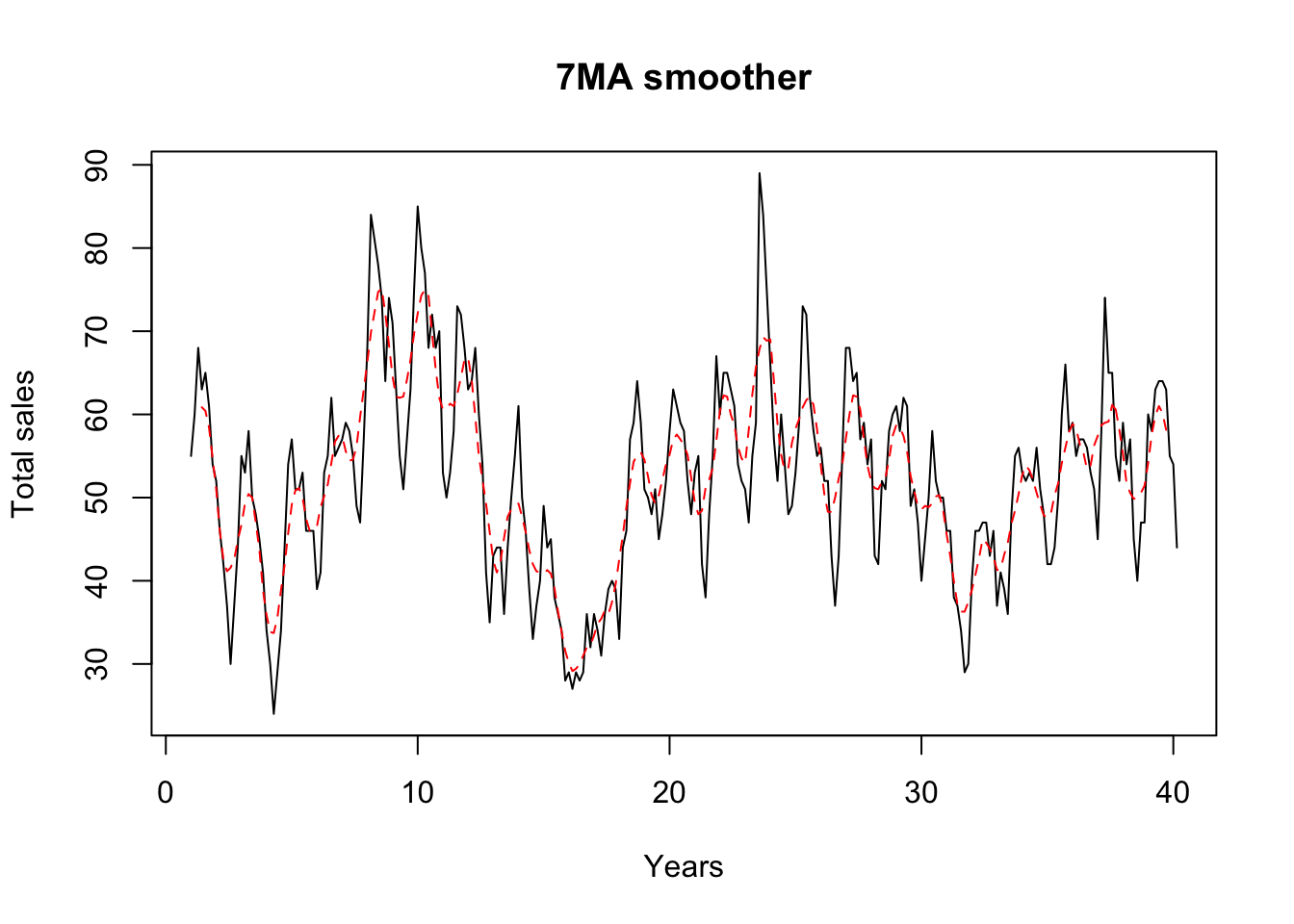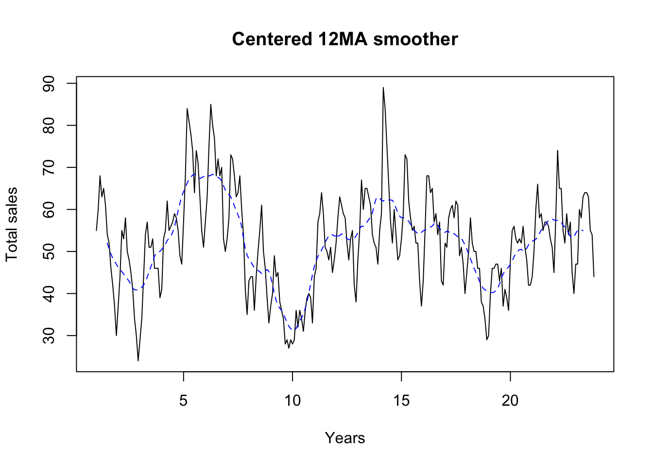

The 7MA tracks the seasonal variation whereas the 2x12MA tracks the cycle without being contaminated by the seasonal variation

Double moving averages

The double moving average works with odd numbers, and can be thought of as the moving average of a moving average. We use the notation $k$ x $k$ MA.
Examples of the 3 MA:

T_{2} = \frac{1}{3} (Y_{1} + Y_{2} + Y_{3}) = \frac{1}{3} (266 + 145.9 + 183.1) = 198.3

T_{3} = \frac{1}{3} (Y_{2} + Y_{3} + Y_{4}) = \frac{1}{3} (145.9 + 183.1 + 119.3) = 149.4

T_{4} = \frac{1}{3} (Y_{3} + Y_{4} + Y_{5}) = \frac{1}{3} (183.1 + 119.3 + 180.3) = 160.9

Example of the 3x3 MA:

\frac{1}{3} (Y_{2} + Y_{3} + Y_{4}) = \frac{1}{3} (198.3 + 149.4 + 160.9) = 169.5

Consider now the weight allocated to each observation using 3x3 MA.

\frac{1}{3} (Y_{2} + Y_{3} + Y_{4}) = \frac{1}{3} (\frac{1}{3} (Y_{1} + Y_{2} + Y_{3}) + \frac{1}{3} (Y_{2} + Y_{3} + Y_{4}) + \frac{1}{3} (Y_{3} + Y_{4} + Y_{5})) = \frac{1}{9} (Y_{1} + 2 Y_{2} + 3 Y_{3} + 2 Y_{4} + Y_{5})

From this we notice that there are five observations, each with a different weight $[\frac{1}{9}; \frac{2}{9}; \frac{3}{9}; \frac{2}{9}; \frac{1}{9}]$ .

Thus, the observations in the middle have higher weights.

Weighted moving averages

Local Regression Smoothing

Loess

#| label: loess
library(readxl)
Shampoo <- read_excel("~/Documents/DataEng/5thYear/Semester 2/Stats 348/Part B/Datasets/Shampoo data.xlsx")
 
Y <- as.numeric(Shampoo[[1]])
 
X <- seq_along(Y)
model<-loess(Y~X,span=0.3,degree=1)
model
 
yhat<-predict(model)

{#output-loess}

Call:
loess(formula = Y ~ X, span = 0.3, degree = 1)

Number of Observations: 35 
Equivalent Number of Parameters: 6.02 
Residual Standard Error: 66.62

#| label: loess_plot
plot(X,Y, main="Shampoo Data")
points(yhat)
points(X,yhat)
plot(X,Y, main="Loess Plot")
lines(X,yhat,col="red")
 
model<-loess(Y~X,span=0.3,degree=2)
yhat<-predict(model)
lines(X,yhat,col="blue")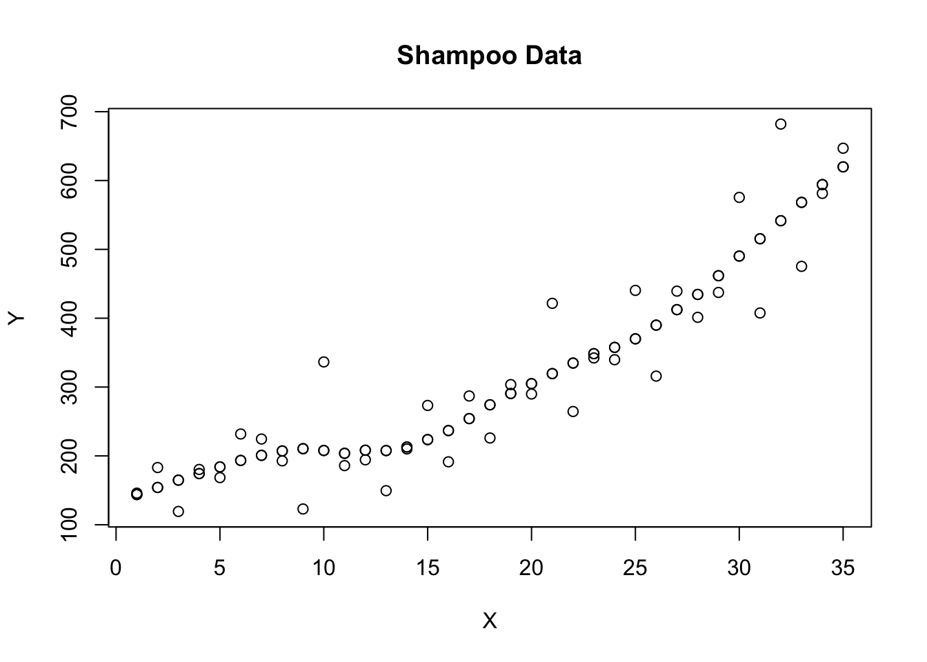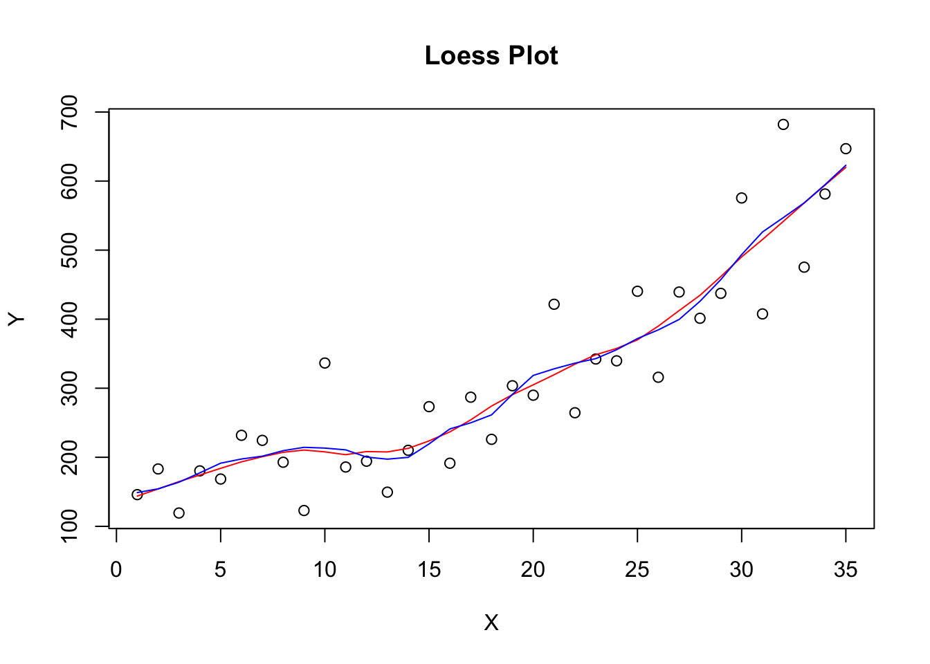

Classical decomposition

Classical decomposition makes use of the moving average. It can be applied to both additive and multiplicative time series.

Additive decomposition

Using the House sales data.xlsx you can decompose the time series into its components (Trend-Cycle, Seasonality, and Irregular components) using the following R commands.

#| label: add_plot
library(readxl)
Sales <- read_excel("~/Documents/DataEng/5thYear/Semester 2/Stats 348/Part B/Datasets/House sales data.xlsx")
Y <- ts(Sales[,2], frequency = 3)
plot(decompose(Y,type="additive"))
 
Y <- ts(Sales[,2], frequency = 12)
plot(decompose(Y,type="additive"))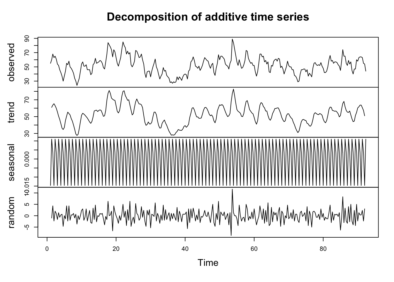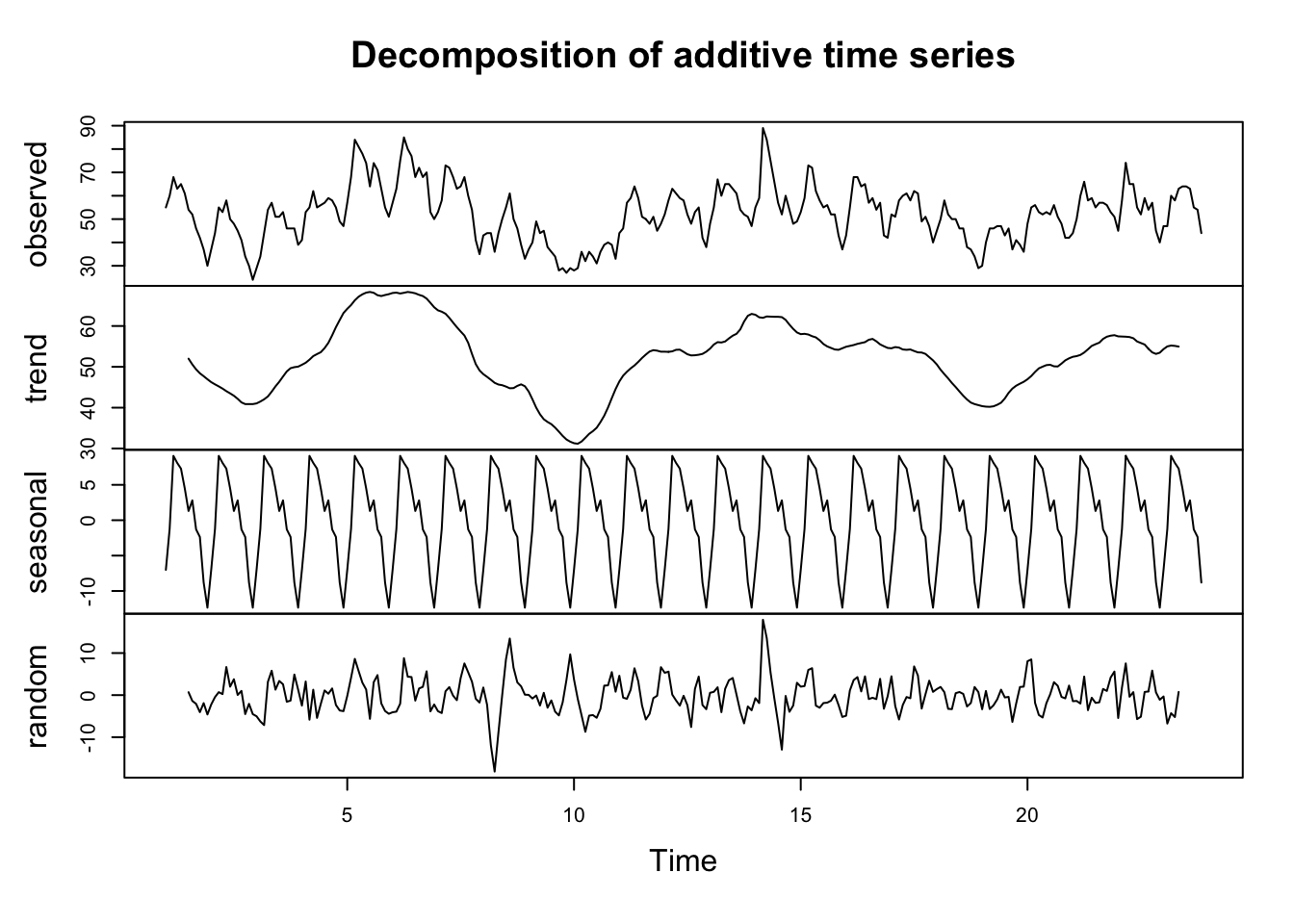

A 3 MA was used to obtain the trend in Figure 1 and a 2x12 Centered moving average was used to obtain the trend in Figure 2.
For the Additive model $Y_{t} = S_{t} + T_{t} + E_{t}$

#| label: add_decompose
output<-decompose(Y,type="additive")
head(output)
 
Yt<-output$x
str(Yt)
St<-output$seasonal
str(St)
Tt<-output$trend
str(Tt)
Et<-output$random
str(Et)

{#output-add_decompose}

$x
   Jan Feb Mar Apr May Jun Jul Aug Sep Oct Nov Dec
1   55  60  68  63  65  61  54  52  46  42  37  30
2   37  44  55  53  58  50  48  45  41  34  30  24
3   29  34  44  54  57  51  51  53  46  46  46  39
4   41  53  55  62  55  56  57  59  58  55  49  47
5   57  68  84  81  78  74  64  74  71  63  55  51
6   57  63  75  85  80  77  68  72  68  70  53  50
7   53  58  73  72  68  63  64  68  60  54  41  35
8   43  44  44  36  44  50  55  61  50  46  39  33
9   37  40  49  44  45  38  36  34  28  29  27  29
10  28  29  36  32  36  34  31  36  39  40  39  33
11  44  46  57  59  64  59  51  50  48  51  45  48
12  52  58  63  61  59  58  52  48  53  55  42  38
13  48  55  67  60  65  65  63  61  54  52  51  47
14  55  59  89  84  75  66  57  52  60  54  48  49
15  53  59  73  72  62  58  55  56  52  52  43  37
16  43  55  68  68  64  65  57  59  54  57  43  42
17  52  51  58  60  61  58  62  61  49  51  47  40
18  45  50  58  52  50  50  46  46  38  37  34  29
19  30  40  46  46  47  47  43  46  37  41  39  36
20  48  55  56  53  52  53  52  56  51  48  42  42
21  44  50  60  66  58  59  55  57  57  56  53  51
22  45  58  74  65  65  55  52  59  54  57  45  40
23  47  47  60  58  63  64  64  63  55  54  44    

$seasonal
          Jan        Feb        Mar        Apr        May        Jun        Jul
1   -7.014159  -1.235750   9.090007   8.095689   7.286977   4.496663   1.304022
2   -7.014159  -1.235750   9.090007   8.095689   7.286977   4.496663   1.304022
3   -7.014159  -1.235750   9.090007   8.095689   7.286977   4.496663   1.304022
4   -7.014159  -1.235750   9.090007   8.095689   7.286977   4.496663   1.304022
5   -7.014159  -1.235750   9.090007   8.095689   7.286977   4.496663   1.304022
6   -7.014159  -1.235750   9.090007   8.095689   7.286977   4.496663   1.304022
7   -7.014159  -1.235750   9.090007   8.095689   7.286977   4.496663   1.304022
8   -7.014159  -1.235750   9.090007   8.095689   7.286977   4.496663   1.304022
9   -7.014159  -1.235750   9.090007   8.095689   7.286977   4.496663   1.304022
10  -7.014159  -1.235750   9.090007   8.095689   7.286977   4.496663   1.304022
11  -7.014159  -1.235750   9.090007   8.095689   7.286977   4.496663   1.304022
12  -7.014159  -1.235750   9.090007   8.095689   7.286977   4.496663   1.304022
13  -7.014159  -1.235750   9.090007   8.095689   7.286977   4.496663   1.304022
14  -7.014159  -1.235750   9.090007   8.095689   7.286977   4.496663   1.304022
15  -7.014159  -1.235750   9.090007   8.095689   7.286977   4.496663   1.304022
16  -7.014159  -1.235750   9.090007   8.095689   7.286977   4.496663   1.304022
17  -7.014159  -1.235750   9.090007   8.095689   7.286977   4.496663   1.304022
18  -7.014159  -1.235750   9.090007   8.095689   7.286977   4.496663   1.304022
19  -7.014159  -1.235750   9.090007   8.095689   7.286977   4.496663   1.304022
20  -7.014159  -1.235750   9.090007   8.095689   7.286977   4.496663   1.304022
21  -7.014159  -1.235750   9.090007   8.095689   7.286977   4.496663   1.304022
22  -7.014159  -1.235750   9.090007   8.095689   7.286977   4.496663   1.304022
23  -7.014159  -1.235750   9.090007   8.095689   7.286977   4.496663   1.304022
          Aug        Sep        Oct        Nov        Dec
1    2.798341  -1.298250  -2.364538  -8.805826 -12.353175
2    2.798341  -1.298250  -2.364538  -8.805826 -12.353175
3    2.798341  -1.298250  -2.364538  -8.805826 -12.353175
4    2.798341  -1.298250  -2.364538  -8.805826 -12.353175
5    2.798341  -1.298250  -2.364538  -8.805826 -12.353175
6    2.798341  -1.298250  -2.364538  -8.805826 -12.353175
7    2.798341  -1.298250  -2.364538  -8.805826 -12.353175
8    2.798341  -1.298250  -2.364538  -8.805826 -12.353175
9    2.798341  -1.298250  -2.364538  -8.805826 -12.353175
10   2.798341  -1.298250  -2.364538  -8.805826 -12.353175
11   2.798341  -1.298250  -2.364538  -8.805826 -12.353175
12   2.798341  -1.298250  -2.364538  -8.805826 -12.353175
13   2.798341  -1.298250  -2.364538  -8.805826 -12.353175
14   2.798341  -1.298250  -2.364538  -8.805826 -12.353175
15   2.798341  -1.298250  -2.364538  -8.805826 -12.353175
16   2.798341  -1.298250  -2.364538  -8.805826 -12.353175
17   2.798341  -1.298250  -2.364538  -8.805826 -12.353175
18   2.798341  -1.298250  -2.364538  -8.805826 -12.353175
19   2.798341  -1.298250  -2.364538  -8.805826 -12.353175
20   2.798341  -1.298250  -2.364538  -8.805826 -12.353175
21   2.798341  -1.298250  -2.364538  -8.805826 -12.353175
22   2.798341  -1.298250  -2.364538  -8.805826 -12.353175
23   2.798341  -1.298250  -2.364538  -8.805826           

$trend
        Jan      Feb      Mar      Apr      May      Jun      Jul      Aug
1        NA       NA       NA       NA       NA       NA 52.00000 50.58333
2  46.25000 45.70833 45.20833 44.66667 44.04167 43.50000 42.91667 42.16667
3  41.04167 41.50000 42.04167 42.75000 43.91667 45.20833 46.33333 47.62500
4  50.50000 51.00000 51.75000 52.62500 53.12500 53.58333 54.58333 55.87500
5  64.20833 65.12500 66.29167 67.16667 67.75000 68.16667 68.33333 68.12500
6  68.08333 68.16667 67.95833 68.12500 68.33333 68.20833 68.00000 67.62500
7  63.83333 63.50000 63.00000 62.00000 60.83333 59.70833 58.66667 57.66667
8  48.20833 47.54167 46.83333 46.08333 45.66667 45.50000 45.16667 44.75000
9  43.95833 42.04167 40.00000 38.37500 37.16667 36.50000 35.95833 35.12500
10 31.29167 31.16667 31.70833 32.62500 33.58333 34.25000 35.08333 36.45833
11 46.41667 47.83333 48.79167 49.62500 50.33333 51.20833 52.16667 53.00000
12 53.70833 53.66667 53.79167 54.16667 54.20833 53.66667 53.08333 52.79167
13 54.45833 55.45833 56.04167 55.95833 56.20833 56.95833 57.62500 58.08333
14 62.75000 62.12500 62.00000 62.33333 62.29167 62.25000 62.25000 62.16667
15 58.00000 58.08333 57.91667 57.50000 57.20833 56.50000 55.58333 55.00000
16 54.91667 55.12500 55.33333 55.62500 55.83333 56.04167 56.62500 56.83333
17 54.54167 54.83333 54.70833 54.25000 54.16667 54.25000 53.87500 53.54167
18 50.58333 49.29167 48.20833 47.16667 46.04167 45.04167 43.95833 42.91667
19 40.37500 40.25000 40.20833 40.33333 40.70833 41.20833 42.25000 43.62500
20 46.95833 47.75000 48.75000 49.62500 50.04167 50.41667 50.50000 50.12500
21 52.45833 52.62500 52.91667 53.50000 54.29167 55.12500 55.54167 55.91667
22 57.45833 57.41667 57.37500 57.29167 57.00000 56.20833 55.83333 55.45833
23 54.33333 55.00000 55.20833 55.12500 54.95833       NA       NA       NA
        Sep      Oct      Nov      Dec
1  49.37500 48.41667 47.70833 46.95833
2  41.29167 40.87500 40.87500 40.87500
3  48.87500 49.66667 49.91667 50.04167
4  57.70833 59.70833 61.45833 63.16667
5  67.54167 67.33333 67.58333 67.79167
6  67.33333 66.70833 65.66667 64.58333
7  55.87500 53.16667 50.66667 49.12500
8  44.79167 45.33333 45.70833 45.25000
9  34.12500 33.08333 32.20833 31.66667
10 38.04167 40.04167 42.33333 44.54167
11 53.75000 54.08333 53.95833 53.70833
12 52.83333 52.95833 53.16667 53.70833
13 59.16667 61.08333 62.50000 62.95833
14 61.50000 60.33333 59.29167 58.41667
15 54.62500 54.25000 54.16667 54.54167
16 56.25000 55.50000 55.04167 54.62500
17 53.50000 53.16667 52.37500 51.58333
18 42.00000 41.25000 40.87500 40.62500
19 44.66667 45.37500 45.87500 46.33333
20 50.08333 50.79167 51.58333 52.08333
21 56.83333 57.37500 57.62500 57.75000
22 54.41667 53.54167 53.16667 53.45833
23       NA       NA       NA         

$random
             Jan           Feb           Mar           Apr           May
1             NA            NA            NA            NA            NA
2   -2.235840548  -0.472582973   0.701659452   0.237644300   6.671356421
3   -5.027507215  -6.264249639  -7.131673882   3.154310967   5.796356421
4   -2.485840548   3.235750361  -5.840007215   1.279310967  -5.411976912
5   -0.194173882   4.110750361   8.618326118   5.737644300   2.963023088
6   -4.069173882  -3.930916306  -2.048340548   8.779310967   4.379689755
7   -3.819173882  -4.264249639   0.909992785   1.904310967  -0.120310245
8    1.805826118  -2.305916306 -11.923340548 -18.179022367  -8.953643579
9    0.055826118  -0.805916306  -0.090007215  -2.470689033   0.546356421
10   3.722492785  -0.930916306  -4.798340548  -8.720689033  -4.870310245
11   4.597492785  -0.597582973  -0.881673882   1.279310967   6.379689755
12   5.305826118   5.569083694   0.118326118  -1.262355700  -2.495310245
13   0.555826118   0.777417027   1.868326118  -4.054022367   1.504689755
14  -0.735840548  -1.889249639  17.909992785  13.570977633   5.421356421
15   2.014159452   2.152417027   5.993326118   6.404310967  -2.495310245
16  -4.902507215   1.110750361   3.576659452   4.279310967   0.879689755
17   4.472492785  -2.597582973  -5.798340548  -2.345689033  -0.453643579
18   1.430826118   1.944083694   0.701659452  -3.262355700  -3.328643579
19  -3.360840548   0.985750361  -3.298340548  -2.429022367  -0.995310245
20   8.055826118   8.485750361  -1.840007215  -4.720689033  -5.328643579
21  -1.444173882  -1.389249639  -2.006673882   4.404310967  -3.578643579
22  -5.444173882   1.819083694   7.534992785  -0.387355700   0.713023088
23  -0.319173882  -6.764249639  -4.298340548  -5.220689033   0.754689755
             Jun           Jul           Aug           Sep           Oct
1             NA   0.695977633  -1.381673882  -2.076749639  -4.052128427
2    2.003336941   3.779310967   0.034992785   1.006583694  -4.510461760
3    1.295003608   3.362644300   2.576659452  -1.576749639  -1.302128427
4   -2.079996392   1.112644300   0.326659452   1.589917027  -2.343795094
5    1.336670274  -5.637355700   3.076659452   4.756583694  -1.968795094
6    4.295003608  -1.304022367   1.576659452   1.964917027   5.656204906
7   -1.204996392   4.029310967   7.534992785   5.423250361   3.197871573
8    0.003336941   8.529310967  13.451659452   6.506583694   3.031204906
9   -2.996663059  -1.262355700  -3.923340548  -4.826749639  -1.718795094
10  -4.746663059  -5.387355700  -3.256673882   2.256583694   2.322871573
11   3.295003608  -2.470689033  -5.798340548  -4.451749639  -0.718795094
12  -0.163329726  -2.387355700  -7.590007215   1.464917027   4.406204906
13   3.545003608   4.070977633   0.118326118  -3.868416306  -6.718795094
14  -0.746663059  -6.554022367 -12.965007215  -0.201749639  -3.968795094
15  -2.996663059  -1.887355700  -1.798340548  -1.326749639   0.114538240
16   4.461670274  -0.929022367  -0.631673882  -0.951749639   3.864538240
17  -0.746663059   6.820977633   4.659992785  -3.201749639   0.197871573
18   0.461670274   0.737644300   0.284992785  -2.701749639  -1.885461760
19   1.295003608  -0.554022367  -0.423340548  -6.368416306  -2.010461760
20  -1.913329726   0.195977633   3.076659452   2.214917027  -0.427128427
21  -0.621663059  -1.845689033  -1.715007215   1.464917027   0.989538240
22  -5.704996392  -5.137355700   0.743326118   0.881583694   5.822871573
23            NA            NA            NA            NA            NA
             Nov           Dec
1   -1.902507215  -4.605158730
2   -2.069173882  -4.521825397
3    4.889159452   1.311507937
4   -3.652507215  -3.813492063
5   -3.777507215  -4.438492063
6   -3.860840548  -2.230158730
7   -0.860840548  -1.771825397
8    2.097492785   0.103174603
9    3.597492785   9.686507937
10   5.472492785   0.811507937
11  -0.152507215   6.644841270
12  -2.360840548  -3.355158730
13  -2.694173882  -3.605158730
14  -2.485840548   2.936507937
15  -2.360840548  -5.188492063
16  -3.235840548  -0.271825397
17   3.430826118   0.769841270
18   1.930826118   0.728174603
19   1.930826118   2.019841270
20  -0.777507215   2.269841270
21   4.180826118   5.603174603
22   0.639159452  -1.105158730
23            NA              

$figure
 [1]  -7.014159  -1.235750   9.090007   8.095689   7.286977   4.496663
 [7]   1.304022   2.798341  -1.298250  -2.364538  -8.805826 -12.353175

$type
[1] "additive"


 Time-Series [1:275, 1] from 1 to 23.8: 55 60 68 63 65 61 54 52 46 42 ...
 - attr(*, "dimnames")=List of 2
  ..$ : NULL
  ..$ : chr "Sales"

 Time-Series [1:275] from 1 to 23.8: -7.01 -1.24 9.09 8.1 7.29 ...

 Time-Series [1:275, 1] from 1 to 23.8: NA NA NA NA NA ...

 Time-Series [1:275, 1] from 1 to 23.8: NA NA NA NA NA ...
 - attr(*, "dimnames")=List of 2
  ..$ : NULL
  ..$ : chr "x - seasonal"

Removing the Trend-Cycle: $Y_{t} - T_{t} = S_{t} + E_{t}$
Removing the Trend-Cycle and Seasonality: $E_{t} = Y_{t} - T_{t} - S_{t}$

Multiplicative decomposition

#| label: multi_plot
library(readxl)
Sales <- read_excel("~/Documents/DataEng/5thYear/Semester 2/Stats 348/Part B/Datasets/House sales data.xlsx")
Sales_df <- as.data.frame(Sales)
Y <- ts(Sales[,2], frequency = 3)
plot(decompose(Y,type="multiplicative"))
 
Y <- ts(Sales[,2], frequency = 12)
plot(decompose(Y,type="multiplicative"))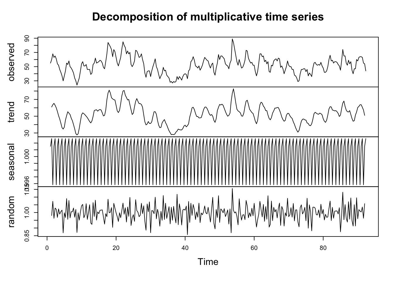

For the Multiplicative model: $Y_{t} = S_{t} \times T_{t} \times E_{t}$

#| label: multi_decompose
output<-decompose(Y,type="multiplicative")
Yt<-output$x
str(Yt)
St<-output$seasonal
str(St)
Tt<-output$trend
str(Tt)
Et<-output$random
str(Et)

{#output-multi_decompose}

Time-Series [1:275, 1] from 1 to 23.8: 55 60 68 63 65 61 54 52 46 42 ...
 - attr(*, "dimnames")=List of 2
  ..$ : NULL
  ..$ : chr "Sales"

 Time-Series [1:275] from 1 to 23.8: 0.865 0.977 1.171 1.149 1.142 ...

 Time-Series [1:275, 1] from 1 to 23.8: NA NA NA NA NA ...

 Time-Series [1:275, 1] from 1 to 23.8: NA NA NA NA NA ...
 - attr(*, "dimnames")=List of 2
  ..$ : NULL
  ..$ : chr "x/seasonal"

Removing the Trend-Cycle: $\frac{Y _{t}}{T _{t}} = S_{t} \times E_{t}$
Removing the Trend-Cycle and Seasonality: $E_{t} = \frac{Y _{t}}{T _{t} S _{t}}$

STL decomposition

STL decomposition makes use of the moving lines (“Seasonal-Trend decomposition procedure based on Loess” - STL).
It is only applied to an additive time series. Thus, if a time series is multiplicative, we take the log to make it additive and then apply STL.
Using the House sales data.xlsx you can decompose the time series into its components (Trend-Cycle, Seasonality, and Irregular components) using the following R commands.

#| label: STL
library(readxl)
Sales <- read_excel("~/Documents/DataEng/5thYear/Semester 2/Stats 348/Part B/Datasets/House sales data.xlsx")
Sales <- as.data.frame(Sales)
Y <- ts(Sales[, 2], frequency = 12)
output<-stl(Y,s.window=20)
plot(output)
head(output[[1]])
 
St<-output[[1]][,1]
Tt<-output[[1]][,2]
Et<-output[[1]][,3]

{#output-STL}

seasonal    trend remainder
[1,] -7.395254 61.14190  1.253357
[2,] -1.656227 59.69365  1.962580
[3,]  8.365473 58.24540  1.389129
[4,]  8.125428 56.79715 -1.922576
[5,]  8.191360 55.44472  1.363924
[6,]  5.019674 54.09228  1.888043